220-ChIP-Seq数据中包含了spike-in怎么分析
刘小泽写于2020.11.27 换个说法就是:一套ChIP-Seq中同时混有两套基因组,一套内源占多数,一套外源占少数 写这一篇,着实收获比较大,看了不知道多少个说明书、文章、网站。。。 其中的每一步都是一点点探索出来的
什么是Chip-Seq中的spike-in
可以参考:https://www.activemotif.com/catalog/1091/chip-normalization
ChIP-Seq方便了在基因组区域对转录因子结合位点以及组蛋白转录后修饰的探索,但技术本身是半定量的,不能准确地比较样本与样本的结合丰度。有一个讲座介绍了这个问题:https://www.activemotif.com/chip-normalization-webinar-request
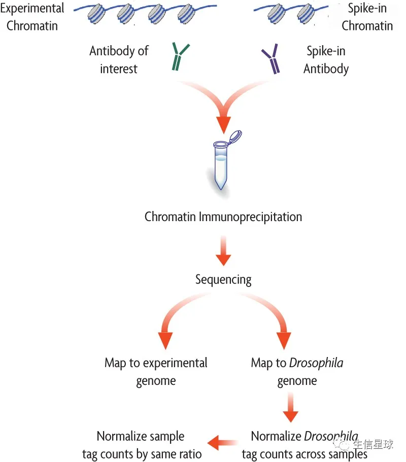
但如果在ChIP实验之前,在所有样本中加入一点外源染色质(它相当于一个恒定的值),即使出现一些技术误差,那么就会体现在spike-in上,后面我们就能通过自己样本去掉spike-in体现的误差,来更好地反应真实的丰度
来自 https://www.ncbi.nlm.nih.gov/pmc/articles/PMC4079971/ 的描述: This method addresses the problem via an experimental procedure conducted prior to immunoprecipitation. It consists of adding a constant, low amount of a single batch of foreign chromatin (e.g., human) as an internal control to each sample of the chromatin of interest (e.g., mouse) before immunoprecipitation.
作用1:Reduce the Effects of Technical Variation
to correct for differences that results from sample loss, amplification bias, uneven sequencing read depth, or hand-to-hand differences between users
作用2:Identify Biological Differences Not Observed by Standard ChIP Analysis
to monitor the effects of experimental conditions, such as inhibitory compounds or mutants to reveal biological differences.
作用3:Specificity of Detection
The Spike-in Antibody shows minimal cross reactivity with mammalian samples. When the Spike-in Antibody was tested in ChIP-Seq with human chromatin, there is little to no signal detected.
整体的思路
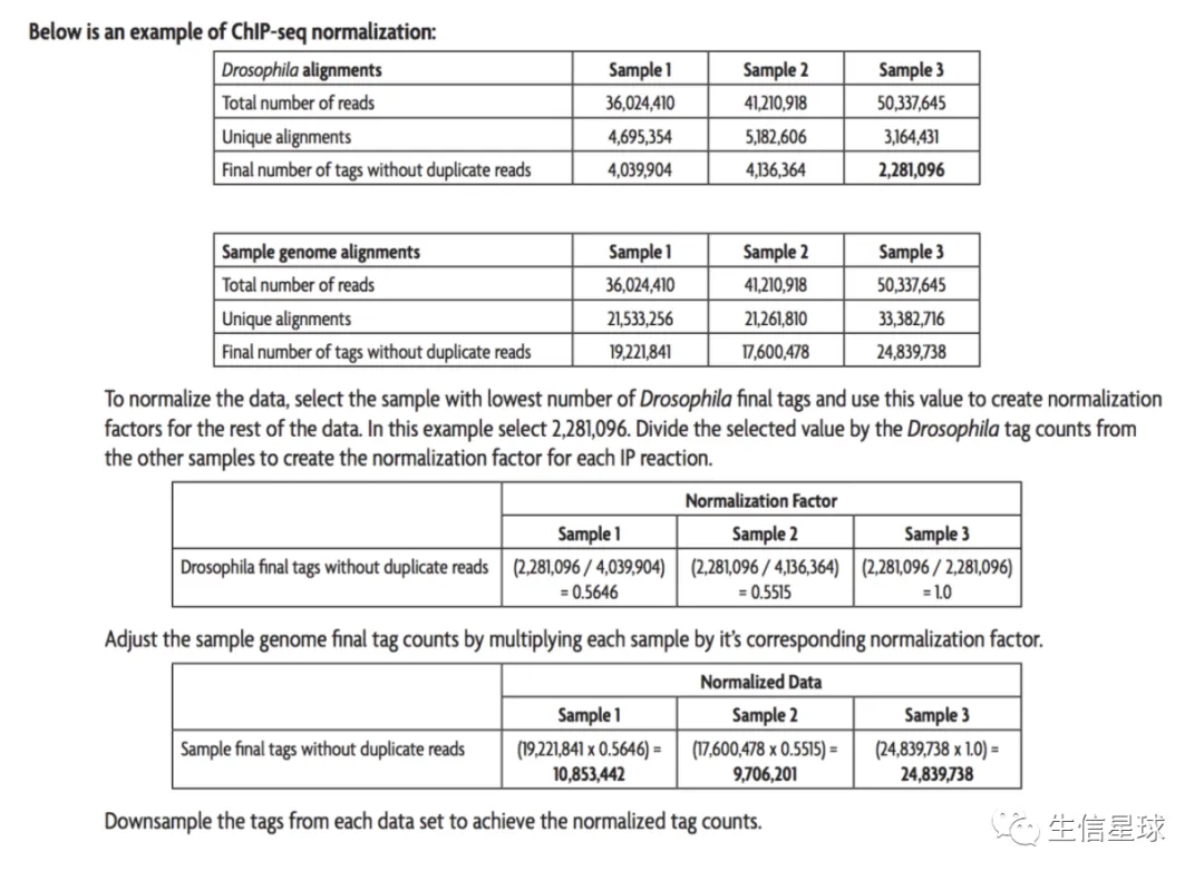
可以这么计算scale factor:
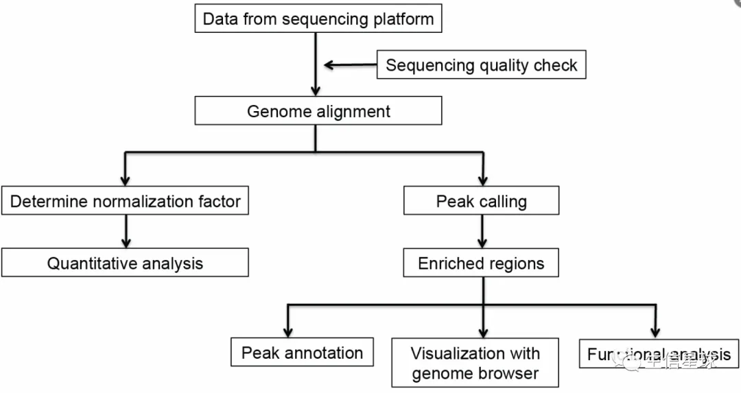
大体步骤
- 根据文章:An Alternative Approach to ChIP-Seq Normalization Enables Detection of Genome- Wide Changes in Histone H3 Lysine 27 Trimethylation upon EZH2 Inhibition的方法描述,先将reads分别比对到不同的基因组,然后去重复,取高质量比对的结果(比如mapping quality > 25)
- 利用
ChIPSeqSpike对外源spike-in计算scale factor - 利用
bamCoverage将bam转为bw,注意加一些参数,比如:--scaleFactor, --extendReads, --effectiveGenomeSize - 接下来就可以对bw进行操作,或者继续call peaks以及寻找差异peaks
在BioProtocol 网站中 (https://bio-protocol.org/e2981) 中也介绍了一些pipeline
它也强调,加入spike-in的场景一般是:
- Traditional ChIP-seq protocols are not inherently quantitative and therefore prohibit direct comparison between samples derived from distinct cell types or cells that have been through different genetic or chemical perturbation
- In 2014, Orlando et al. (2014) developed a method, called ChIP with reference exogenous genome (ChIP-Rx), which utilizes a constant amount of reference or ‘‘spike-in’’ epigenome for cell-based comparison among epigenomes.
原始数据质控
reads比对:分别比对到内源和外源两个参考基因组,并对内源的bam排序+构建索引
得到scale factor:
第一步:将内源和外源的比对reads合并,作为 每个样本的total mapped reads ,并且规定
# 这里mm是外源,dm是内源
α = the spike-in scale factor
β = the histone modification level
γ = the percentage of input mouse reads in total input mapped reads
Nm = the number of mouse mapped reads (in millions) in IP sample
Nd = the number of Drosophila mapped reads (in millions) in IP sample
第二步:计算spike-in scale factor:
α = γ/Nm第三步:计算histone modification level :
β = Nd x α第四步:利用deeptools将内源比对bam进行scale
bamCoverage -b {sample}_ChIP_dm6_Sorted.bam -o {sample}_ChIP_dm6_scaleFactor.bw –scaleFactor α -bs 10 -p 2 –v
定量分析:用
Bwtool计算每个基因区间的ChIP intensitybwtool summary {gene}.bed {sample}_ChIP_dm6_scaleFactor.bw {sample}_{gene}_summary.xls –header**Peak calling:**利用
homer# step1 makeTagDirectory {sample}_ChIP_tag -fragLength 200 {sample}_ChIP.sam -single # step2 makeTagDirectory {sample}_input_tag -fragLength 200 {sample}_input.sam -single # step3 findPeaks {sample}_ChIP_tag/ -style histone -o {sample}_size3K_Peaks.xls -i {sample}_input_tag/ -F 2 -size 3000 -minDist 5000 -fragLength 200Peak可视化:IGV可视化
bamCoverage得到的bw文件Peak注释:同样可以用
homer的annotatePeaksannotatePeaks.pl peaks.txt dm6.bed > annotatedPeaks.txt画图:可以用
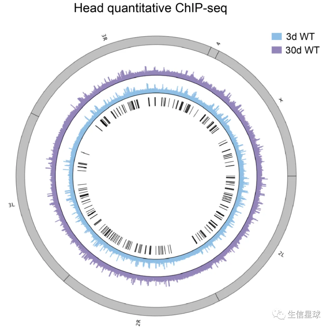
J-circos-V1对bw文件画圈圈图,更好地展示H3K27me3的peaks分布- Black boxes and lines (innermost circle) represented common peak regions
- Chromosome ideogram was in grey (outermost ring)
1 比对
cat $config |while read i
do
  	# echo $i
    conf=($i)
  	sample=${conf[1]}

    fq1=$wkd/clean/${sample}.fq1.gz
    fq2=$wkd/clean/${sample}.fq2.gz

    ## step1: align mouse
    if [  ! -f  log/${sample}.mm.bowtie2.done ]; then
      	bowtie2  -p 4  --local --very-sensitive-local \
      		--no-mixed --no-unal --no-discordant \
      		-q --phred33 \
      		-x $mm_index -1 $fq1 -2 $fq2 2> log/log.bowtie2.mm.${sample}.txt| \
      	samtools view -bhS -q 25 - | \
      	samtools sort  -O bam  -@ 4 -o - > align/${sample}.mm.bam
    fi
    if [ $? -eq 0 ]; then
             touch  log/${sample}.mm.bowtie2.done
          else
             touch log/${sample}.mm.bowtie2.failed
    fi

    # remove duplicate
    if [  ! -f log/${sample}.mm.sambamba.done ]; then
          sambamba markdup  -r  align/${sample}.mm.bam align/${sample}_rm.mm.bam && \
          samtools index align/${sample}_rm.mm.bam
    fi
    if [ $? -eq 0 ]; then
             touch  log/${sample}.mm.sambamba.done
          else
             touch log/${sample}.mm.sambamba.failed
    fi

    ## step2: align human
    if [  ! -f  log/${sample}.hg.bowtie2.done ]; then
      	bowtie2  -p 4  --local --very-sensitive-local \
      		--no-mixed --no-unal --no-discordant \
      		-q --phred33 \
      		-x $hg_index -1 $fq1 -2 $fq2 2> log/log.bowtie2.hg.${sample}.txt| \
      	samtools view -bhS -q 25 - | \
      	samtools sort  -O bam  -@ 4 -o - > align/${sample}.hg.bam
    fi
    if [ $? -eq 0 ]; then
             touch  log/${sample}.hg.bowtie2.done
          else
             touch log/${sample}.hg.bowtie2.failed
    fi

    # remove duplicate
    if [  ! -f log/${sample}.hg.sambamba.done ]; then
          sambamba markdup  -r  align/${sample}.hg.bam align/${sample}_rm.hg.bam && \
          samtools index align/${sample}_rm.hg.bam
    fi
    if [ $? -eq 0 ]; then
             touch  log/${sample}.hg.sambamba.done
          else
             touch log/${sample}.hg.sambamba.failed
    fi

done
2 使用ChIPSeqSpike
官网在:https://www.bioconductor.org/packages/release/bioc/html/ChIPSeqSpike.html
Spike-in normalization procedure consists of 4 steps: RPM scaling, input DNA subtraction, RPM scaling reversal and exogenous spike-in DNA scaling
输入文件(info_file_csv)如下:

- expName:样本名称
- endogenousBam:处理样本比对到内源参考基因组的bam
- exogenousBam:处理样本比对到外源(spike-in)参考基因组的bam
- inputBam:input样本比对到内源参考基因组的bam
- bigWigEndogenous:处理样本比对到内源参考基因组得到的bw
- bigWigInput:input样本比对到内源参考基因组得到的bw
还需要bam、bw文件的位置信息
csds_test <- spikeDataset(info_file_csv, bam_path, bigwig_path)
is(csds_test)
## [1] "ChIPSeqSpikeDatasetList"
示例代码
# BiocManager::install('ChIPSeqSpike')
suppressMessages(library('ChIPSeqSpike'))
# 加载示例数据
info_file_csv <- system.file("extdata/info.csv", package="ChIPSeqSpike")
info_file <- read.csv(info_file_csv)
head(info_file)
bam_path <- system.file("extdata/bam_files", package="ChIPSeqSpike")
bigwig_path <- system.file("extdata/bigwig_files", package="ChIPSeqSpike")


csds_test <- spikeDataset(info_file_csv, bam_path, bigwig_path)
is(csds_test)
csds_test <- estimateScalingFactors(csds_test, verbose = FALSE)
## Scores on testing sub-samples
# Scaling factor is defined as 1000000/bam_count
# 结果返回bam counts以及endogenous/exogenous scaling factors for all experiments
spikeSummary(csds_test)

# the percentage of exogenous DNA
# 一般来讲外源DNA比例(相对于内源)应该在2-25%之间。多一点不会影响normalization,而如果少于2%就会影响
getRatio(csds_test)

# 1: RPM(Reads Per Million scaling
csds_test <- scaling(csds_test)

# 2:Input Subtraction
csds_test <- inputSubtraction(csds_test)

# 3:RPM scaling reversal
csds_test <- scaling(csds_test, reverse = TRUE)

# 4:Exogenous scaling
csds_test <- scaling(csds_test, type = "exo")
- 需要注意:
estimateScalingFactors这里默认是单端数据paired=F,如果你的数据是双端的,会报错,设置成paired=T就可以了 - 提供的bw需要保证起始、终止坐标一致,因为在
inputSubtraction这一步需要用处理组减去input组。如果使用bamCoverage转换的bw,就会遇到坐标不一致的情况,这是因为deepTools会将测序深度一致的相邻bins进行合并,以节省文件空间,当然合并后的坐标就不一致了【即使自己设定了--binSize也不能保证一致】(https://github.com/deeptools/deepTools/issues/907) 这波操作可以看之前的推送: bam转bigwig的binsize问题,你遇到了吗? - 需要保证这里的bw文件是没有经过任何normalized的,因此在使用
bamCoverage时,不需要设置参数--normalizeUsing
最后,每运行一步,都会得到一个新的bw
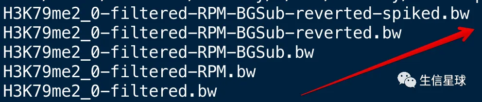
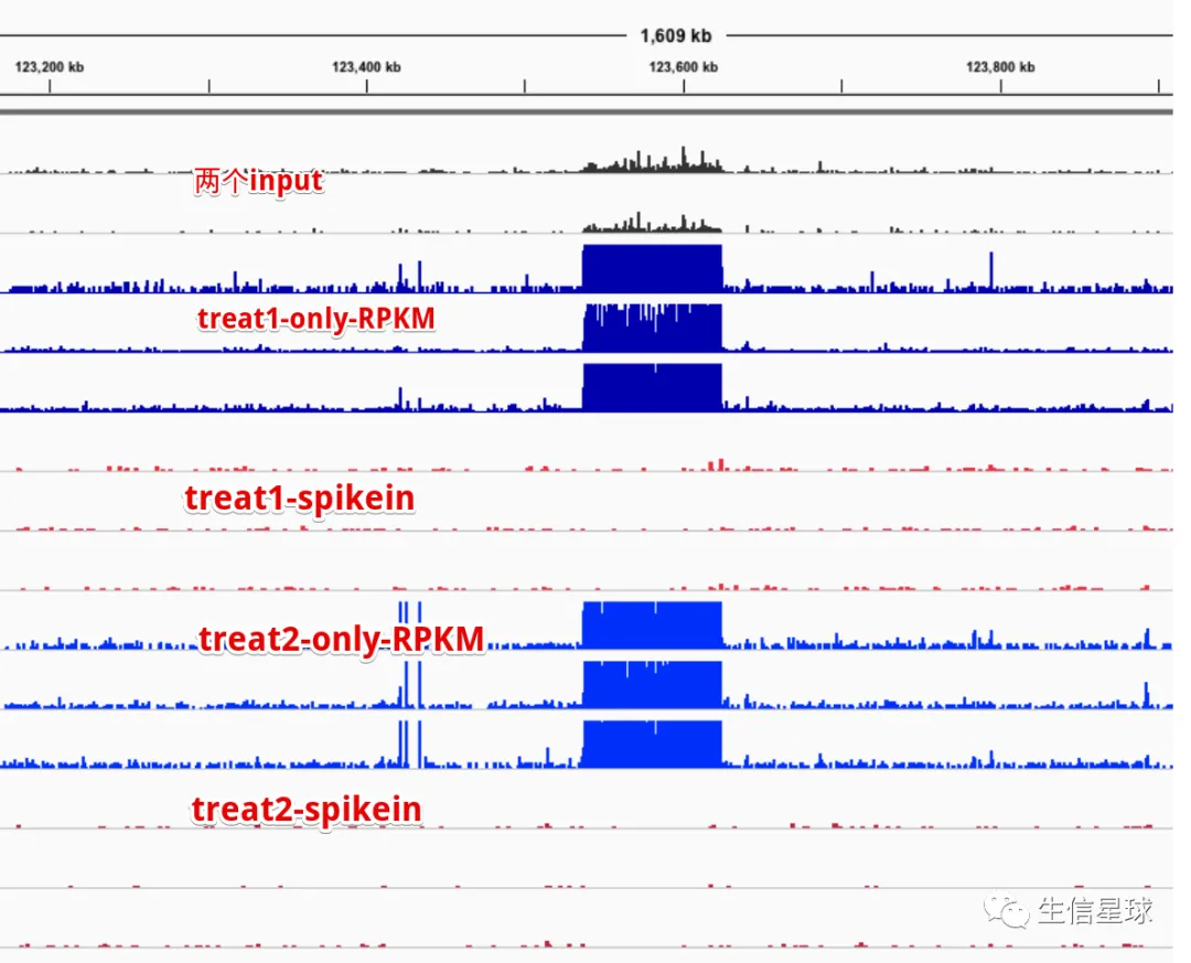
放在IGV中看看
看来spike-in确实可以过滤掉很多影响因素
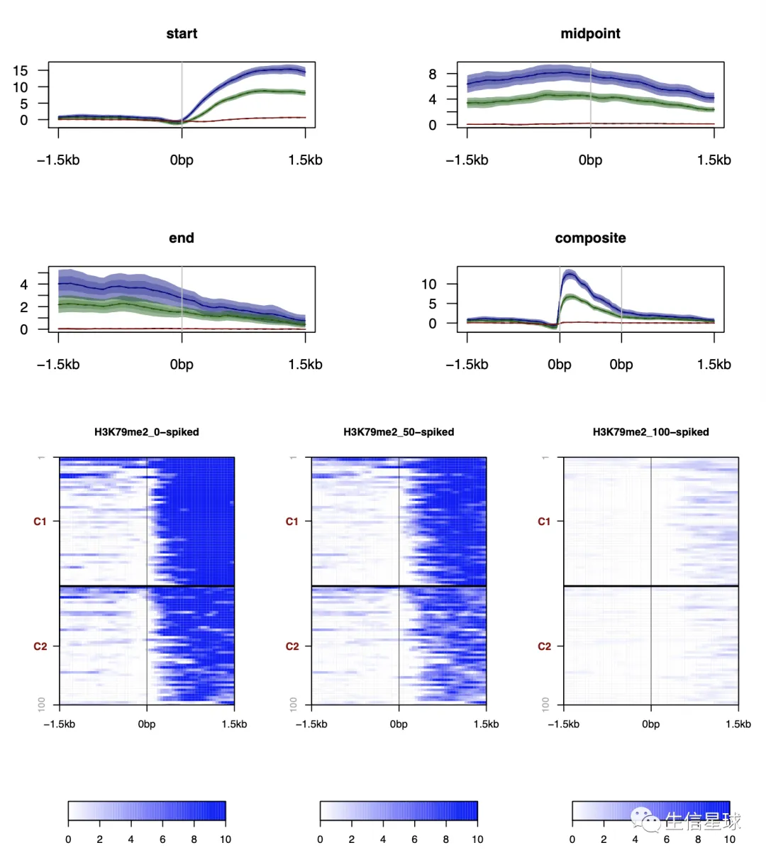
还可以作图
官方文档后面还附带了很多图,很多都是基于这些bw文件,比如
# profiles
plotProfile(csds, legend = TRUE)

# Heatmaps
plotHeatmaps(csds, nb_of_groups = 2, clustering_method = "kmeans")
3 拿到peaks:使用MACS2
使用macs2进行call peaks,最常用的输入文件就是bam
需要注意,如果是双端数据需要设置BAMPE 。软件默认是只保留 5’ 端的 reads,然后构建模型时向3’端移动;如果使用了这个参数,就会跳过构建双峰模型,而是根据实际的插入片段大小来构建峰。与此同时,另外两个参数--nomodel与--extsize 会无效
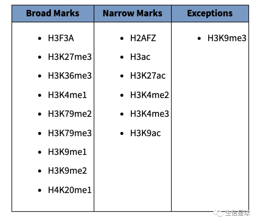
另外,根据组蛋白类型的不同,call peaks的参数设定也不同:
- H3K9me3 is an exception as it is enriched in repetitive regions of the genome.
# CHIP_H3K27me3_T55A_2i_rm.mm.bam
# CHIP_H3K27me3_T55A_SL_rm.mm.bam
# ...
ls CHIP_*bam | cut -d "_" -f 3,4 | while read i;do

	macs2 callpeak -B -g mm -q 0.0001 -f BAMPE -t CHIP_H3K27me3_${i}_rm.mm.bam -c INPUT_${i}_rm.mm.bam -n H3K27me3_${i} --broad --outdir  ../peaks

done
可以对peaks进行统计
# FRiP(Fraction of reads in peaks),peaks中的reads与总reads的比例,即文库中结合位点片段占背景reads的比例,可理解为“信噪比”

## peak峰的个数
Peak_number=`wc -l H3K27me3_T55A_2i_peaks.broadPeak | cut -d ' ' -f1`
## 峰顶的个数
Summit_number=`cut -f1-3 H3K27me3_T55A_2i_peaks.broadPeak|sort -u |wc -l`
## 峰平均长度
cut -f1-3 H3K27me3_T55A_2i_peaks.broadPeak|awk -F '\t' 'BEGIN{sum=0}{sum+=$3-$2}END{print("%.2f\n",sum/'"$Peak_number"')}'

# Calculate FRiP
Total_reads=`samtools view -c  -F 0x0100 CHIP_H3K27me3_T55A_2i_rm.mm.bam` &&\
Peak_reads=`samtools view -c -L H3K27me3_T55A_2i_peaks.broadPeak -F 0x0100 CHIP_H3K27me3_T55A_2i_rm.mm.bam` &&\
echo "scale=4; 100*$Peak_reads/$Total_reads" | bc | awk '{print "FRiP(%)""\t"$1}'
4-1 找差异peaks:MACS2
拿到treat和control的两个指标
然后就可以利用上面👆-B参数得到的.bdg文件了
NAME_treat_pileup.bdgfor treatment dataNAME_control_lambda.bdgfor control
这时如果要对比CHIP_H3K27me3_T55A_2i_rm.mm.bam和CHIP_H3K27me3_T55A_SL_rm.mm.bam,就分别获取fragments after filtering
egrep "fragments after filtering in treatment|fragments after filtering in control" H3K27me3_T55A_2i_peaks.xls
# fragments after filtering in treatment: 1331877
# fragments after filtering in control: 1565909

egrep "fragments after filtering in treatment|fragments after filtering in control" H3K27me3_T55A_SL_peaks.xls
# fragments after filtering in treatment: 3915560
# fragments after filtering in control: 5382520

# actual effective depths of condition 1 and 2 are: 1565909 and 5382520
使用macs2 bdgdiff
macs2 bdgdiff --t1 H3K27me3_T55A_2i_treat_pileup.bdg --c1 H3K27me3_T55A_2i_control_lambda.bdg --t2 H3K27me3_T55A_SL_treat_pileup.bdg \
--c2 H3K27me3_T55A_SL_control_lambda.bdg --d1 1565909 --d2 5382520 --o-prefix diff_T55A_2i_vs_T55A_SL --outdir diff_peaks
# 其中-d1和-d2的值就是运行时输出的reads数目
# 运行成功后,会产生3个文件 diff_c1_vs_c2_c3.0_cond1.bed; diff_c1_vs_c2_c3.0_cond2.bed; diff_c1_vs_c2_c3.0_common.bed
# diff_T55A_2i_vs_T55A_SL_c3.0_cond1.bed保存了在T55A_2i中上调的peak
# diff_T55A_2i_vs_T55A_SL_c3.0_cond2.bed保存了在T55A_SL中上调的peak
# diff_T55A_2i_vs_T55A_SL_c3.0_common.bed文件中保存的是没有达到阈值的,非显著差异peak
# -C: logLR cutoff 默认阈值为3
可以看下结果
$ head -n6 diff_T55A_2i_vs_T55A_SL_c3.0_cond1.bed

track name="condition 1 (peaks)" description="unique regions in condition 1" visibility=1
chr1	71899383	71899635	diff_T55A_2i_vs_T55A_SL_cond1_1	12.11427
chr1	80266819	80267287	diff_T55A_2i_vs_T55A_SL_cond1_2	32.75181
chr1	80322853	80323053	diff_T55A_2i_vs_T55A_SL_cond1_3	10.48444
chr10	78763807	78764061	diff_T55A_2i_vs_T55A_SL_cond1_4	10.84859
chr10	126391854	126392062	diff_T55A_2i_vs_T55A_SL_cond1_5	10.84859
但是,出现一个问题:只能检测出一个样本的富集peaks,另一个是空的

问题来了:bdgdiff能不能进行broad peaks的差异分析?
来自https://www.biostars.org/p/274094/的回答
bdgdiff is not suitable for calling differential broad peaks.
另外在https://www.biostars.org/p/269097/ 也看到有人讨论:
另一款软件
MMDiffseems specific for calling sharp peaks还贴心列举了很多相关软件:
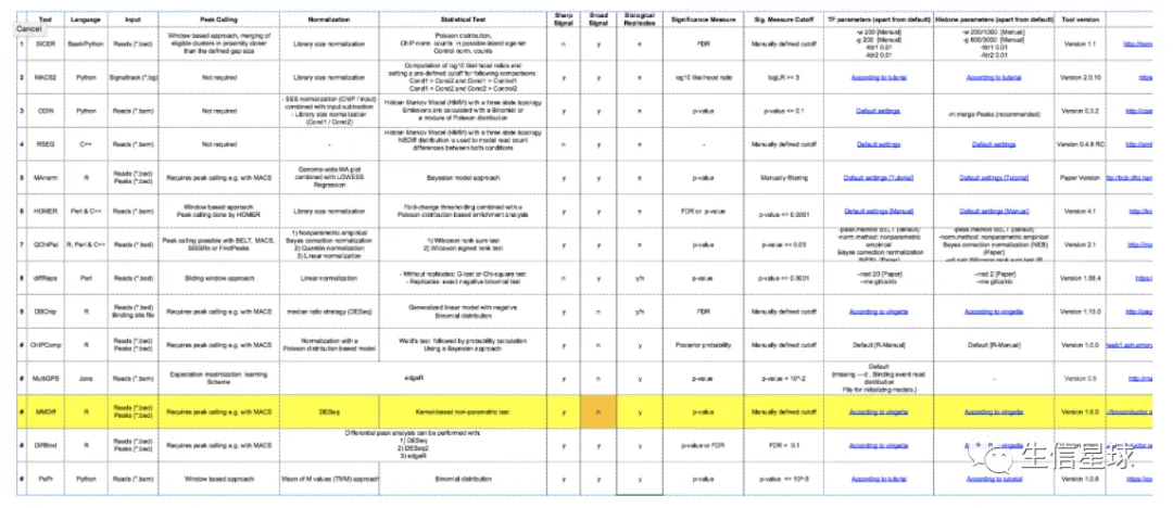
If you have replicates,
DiffBindis a really useful R package that make differential peak calling pretty straightforward.If you don’t have replicates,
MAnormis also useful for directly comparing two samples.
还有一篇文献讨论了这个问题
题目是:An introduction to computational tools fordifferential binding analysis with ChIP-seq data
地址是:http://bioinfo.sibs.ac.cn/shaolab/pdf/2017%20quantitative%20biology;%20review%20of%20chipseq%20differential%20binding%20analysis.pdf
结论是:
- 如果已经有了peaks结果,但是没有生物学重复,可以用MAnorm或者GFOLD软件;
- 如果已经有了peaks结果,而且也有生物学重复,表达量的值还是raw count类型的,那么可以用常用的edgeR, DESeq进行差异分析
- 如果已经有了peaks结果,而且也有生物学重复,表达量的值不是raw count类型的,可以用DBChip, ChIPComp, voom来进行分析
4-2 找差异peaks:DiffBind (有样本重复)
需要注意:所有的样本最好要有生物重复,才能进行有意义的差异分析(看:https://www.biostars.org/p/404289/)
- 解答一:There are no statistically reliable methods that can be used to find differential peaks without replicates.
- 解答二:Replicates are required to do any kind of statistical analysis. Replicates are required to estimate the variance in the data and calculate confidence statistics such as p-values/FDRs.
Without replicates, you can do some exploratory analysis of overlapping peaks (occupancy analysis). For example using
dba.plotVenn().
在https://support.bioconductor.org/p/125809/ 提到了:
Without replicates, you can do some exploratory analysis of overlapping peaks (occupancy analysis). For example using dba.plotVenn(). But not knowing if your data represents an outlier, combined with the inherent noisiness of peak calling, means you will have to have another way to validate any “differential” peaks you identify.
- No replicates: assume simple Poisson model
- With replicates: perform differential test using DE tools from RNA-seq(EdgeR, DESeq,…) based on read counts
4-3 找差异peaks:MAnorm(无样本重复)
软件说明文档在:https://manorm.readthedocs.io/en/latest/
能做什么?
- Comparison of ChIP-Seq data sets of TFs (transcription factors) or epigenetic modifications
- Normalization of two ChIP-seq samples
- Quantitative comparison (differential analysis) of two ChIP-seq samples
- Evaluating the overlap enrichment of the protein binding sites (peaks)
- Elucidating underlying mechanisms of cell-type specific gene regulation
软件安装
conda install -c bioconda manorm
运行
# --p1 --p2 --r1 --r2 -o是5个必须参数
manorm
--p1 sample1_peaks.xls
--p2 sample2_peaks.xls
--pf macs2  # --peak-format (默认bed)
--r1 sample1_reads.bam
--r2 sample2_reads.bam
--rf bam # --read-format (BED,BEDPE,SAM/BAM)
--pe  #paired-end模式
-o output_dir
注意
- 使用
bed格式,会使用到chrom,start,end三列 - 使用
masc2格式时,使用到chrom,start,endandsummit四列。但不与MACS2的broad模式兼容
输出结果
最重要的结果就是:<name1>_vs_<name2>_all_MAvalues.xls
其中的坐标都是1-based的,包含以下信息
- chr: chromosome name
- start: start position of the peak
- end: end position of the peak
- summit: summit position of the peak (absolute position)
- m_value: M value (log2 fold change) of normalized read densities under comparison
- a_value: A value (average signal strength) of normalized read densities under comparison
- p_value
- peak_group: indicates where the peak is come from and whether it is a common peak
- normalized_read_density_in_name1
- normalized_read_density_in_name2
数据测试
# --pf(peak-format) (默认bed)
# --rf(read-format) (BED,BEDPE,SAM/BAM)
# --pe paired-end模式
manorm --p1 peaks/H3K27me3_T55A_2i_peaks.broadPeak --p2 peaks/H3K27me3_T55A_SL_peaks.broadPeak --pf bed  --r1 align/CHIP_H3K27me3_T55A_2i_rm.mm.bam --r2 align/CHIP_H3K27me3_T55A_SL_rm.mm.bam --rf bam  --pe  -o diff_peaks --n1 T55A_2i --n2 T55A_SL
运行日志
==== Running ====
Step 1: Loading input data
Loading peaks of sample 1
Loading peaks of sample 2
Loading reads of sample 1
Loading reads of sample 2
Step 2: Processing peaks
Step 3: Testing the enrichment of peak overlap
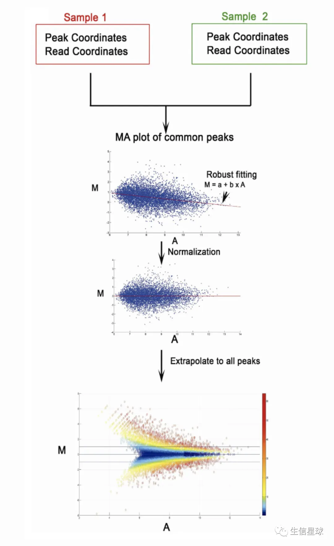
Step 4: Fitting M-A normalization model on common peaks
Step 5: Normalizing all peaks
Step 6: Write output files
==== Stats ====
Total read pairs of sample 1: 1,332,056
Total read pairs of sample 2: 3,915,637
Total peaks of sample 1: 70 (unique: 66 common: 4)
Total peaks of sample 2: 50 (unique: 46 common: 4)
Number of merged common peaks: 4
M-A model: M = 0.84837 * A -4.34602
45 peaks are filtered as unbiased peaks
58 peaks are filtered as sample1-biased peaks
6 peaks are filtered as sample2-biased peaks
看一下结果
# 也就是上面运行日志给出的信息
cat diff_peaks/T55A_2i_vs_T55A_SL_all_MAvalues.xls | sed '1d' |cut -f8| sort | uniq -c
      4 merged_common
     66 T55A_2i_unique
     46 T55A_SL_unique
接下来,可以分别提取出sample1和sample2的unique peaks,进行注释
s1=T55A_2i
s2=T55A_SL

grep ${s1}  T55A_2i_vs_T55A_SL_all_MAvalues.xls >diff_peaks/${s1}_uniq_peaks.txt
grep ${s2}  T55A_2i_vs_T55A_SL_all_MAvalues.xls >diff_peaks/${s2}_uniq_peaks.txt

# anno diff peaks
  	annotatePeaks.pl diff_peaks/${s1}_uniq_peaks.txt mm10 > diff_peaks/${s1}_homer_anno.xls

  	annotatePeaks.pl diff_peaks/${s2}_uniq_peaks.txt mm10 > diff_peaks/${s2}_homer_anno.xls
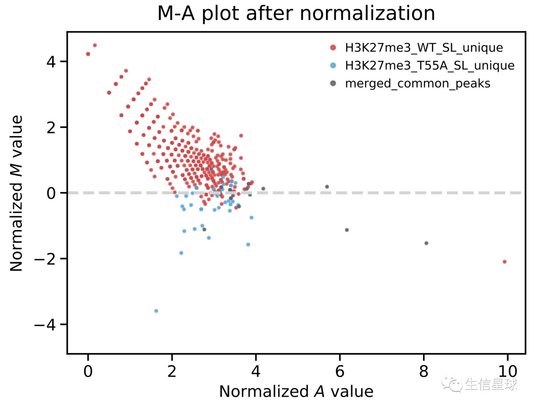
另外,还会得到M-A plot
The M value in MAnorm is the log2 fold change of normalized read densities between sample 1 and sample 2, which quantitatively indicates the difference of the ChIP-seq signal in a specific peak region. The A value is the averaged read density of two ChIP-seq samples under comparison.