227-学一学DNA甲基化芯片分析流程

Jan 14, 2021 12 min read cnposts

刘小泽写于2021.1.14
我学甲基化没啥目的，只是因为好奇目前DNA甲基化有大量的学习资源，既然工具不需要重复造轮子，那么整理过很多遍的背景知识也是一样，以最快吸收为宗旨

背景知识很重要

脱氧核糖的碳编号与碱基的碳编号不要搞混

DNA（脱氧核糖核酸）的主链是由糖+磷酸根重复堆叠而成，在脱氧核糖结构中，将位于氧原子右边的碳原子定义为1号碳，依次排序直至CH2OH的碳原子为5号。

磷酸根连接在糖分子的第5个碳原子的-OH基团上

当然，在形成DNA的过程中，除了糖+磷酸，还需要4种碱基

而碱基的碳原子排序是：

表观遗传与甲基化

来自： DNA 甲基化| Cell Signaling Technology

表观遗传学变化会影响基因活性或表达，但不会以任何方式改变 DNA 序列。

组蛋白和 DNA 会通过以下一系列蛋白出现表观遗传修饰或标记：1) 通过添加表观遗传标记来诱导变化（写入蛋白, writer）；2) 移除表观遗传标记来改变现有状态（擦除蛋白, eraser），或对特定表观遗传标记有反应（读取蛋白, reader）。有很多组表观遗传修饰：乙酰化、甲基化、磷酸化和泛素化。

DNA 甲基化通常与基因沉默有关【但也分区域】
组蛋白上的甲基化标记与基因激活和沉默有关

什么是DNA甲基化？

来自：一文读懂DNA甲基化及BS-seq

DNA甲基化是一个生物过程，它会在在DNA分子中引入甲基化基团，但是甲基化并不会改变序列本身，而会改变DNA片段的活性。最常见的是在胞嘧啶的5号碳位置，在酶和底物的作用下，引入一个甲基基团，变成了5甲基胞嘧啶（5mC），从而改变了它的活性。

怎么定义碱基中的5号碳呢？

CpG是胞嘧啶（C，Cytosine），磷酸（p，phosphoric acid），鸟嘌呤（G，Guanine ）的缩写，也可以去掉磷酸直接叫CG。在哺乳动物中，基因组中富含GC和CpG的序列区段，叫CpG岛（CpG islands）。Regions of the genome that are enriched for non-methylated CpGs, called CpG islands.

CpG岛有几个特征：长度大于200bp、G+C含量高于50%、观察到的CpG与预期CpG的比率大于0.6。

除重复序列外，人类基因组中约有25,000个CpG岛，其中75％的岛长小于850bp
大约50％的CpG岛位于基因启动子区域，而另外25％的岛位于基因内，通常充当替代启动子
人类中大约60-70％的基因在其启动子区域中具有CpG岛，大多数CpG岛在结构上未甲基化

甲基化与基因转录的关系

启动子区域的甲基化与基因表达呈负相关。一方面，DNA本身的甲基化可能在物理上阻碍转录因子与基因的结合；另一方面，甲基化的DNA可以结合甲基CpG结合域（methyl-CpG-binding domain，MBD）这个蛋白，然后MBD又将其他蛋白募集到位点，形成致密的，无活性的异染色质。
基因内的DNA甲基化与基因表达正相关。基因内甲基化似乎与H3K36甲基化紧密相关
from Cancer Cell: Several reports have suggested that gene body DNA methylation may increase transcriptional activity by blocking the initiation of intragenic promoters or by affecting the activities of repetitive DNAs within the transcriptional unit.

来自：甲基化的一些基础知识

DNA甲基化是表观遗传学领域一个重要的研究方向，真核生物中最常见的DNA修饰非5-甲基胞嘧啶（5mC）莫属了，然而在原核生物中最常见的DNA修饰方式则为N6-methyladenine (6mA)，即腺嘌呤第6位氮原子甲基化修饰。

人类是真核生物，所以主要是5mC的DNA甲基化形式。人的参考基因组约30亿碱基，上面不到**1%**是 CpG位点，可以被甲基化，也就是说不到3千万个 CpG 位点。这些 CpG 位点中，大约 60~80% 被甲基化。主要是启动子等特殊区域存在未被甲基化的CpG 岛，那些区域的CpG 位点比较富集。目前研究表明，肿瘤细胞的甲基化水平平均是低于正常细胞的。

DNA甲基化一般与基因沉默相关联。甲基化并非基因沉默的原因而是基因沉默的结果，其以某种机制识别沉默基因，后进行甲基化
非甲基化一般与基因的活化相关联
而去甲基化往往与一个沉默基因的重新激活相关联

来自：我是如何发现850K甲基化芯片和EPIC的区别

850K甲基化芯片和EPIC是同一个芯片的不同表述而已：

Illumina公司提供了一个更强大的甲基化分析平台：Illumina InfiniumMethylationEPIC BeadChip （DNA甲基化850K芯片），不但包含了原450K芯片90%以上的位点，并额外增加了增强子区的350,000个位点，可以对正常样本和FFPE样本单个CpG位点进行定量甲基化检测，该芯片是目前最适合甲基化图谱分析研究的全基因组DNA甲基化芯片。
850K芯片覆盖了全基因组853,307个CpG位点，全面覆盖CpG岛、启动子、编码区及增强子。覆盖CpG岛、RefSeq基因、ENCODE开放染色质、ENCODE转录因子结合位点、FANTOM5增强子区域。

如何检测DNA甲基化？

来自： DNA甲基化技术介绍及发展趋势

1992年BS作为甲基化的金标准定下来之后，在二代测序未出现之前主要是对于位点检测的焦磷酸测序。
2005年二代测序出现后，基于抗体富集方法的MeDIP-seq和经典RRBS出现了
2009年全基因组甲基化出现，但是当时的测序运用并不是很成熟，大多是基于MeDIP做的。
2009：the HumanMethylation27 (27k) array (Bibikova et al. 2009) measured methylation at approximately 27,000 CpGs, primarily in gene promoters. Like bisulfite sequencing, the Infinium assay detects methylation status at single base resolution.
2010年HiSeq 2000出现才开始BS金标准的方法去尝试WGBS、RRBS的改进，然而也没有解决甲基化技术和成本的问题，直到HiSeq X10出现，降低了测序成本，国内才开始推出WGBS。
目前主流的是RRBS、WGBS和Illumina的450k、850K芯片

来自：多分组的甲基化差异分析之QDMR、初识DNA甲基化芯片

**全基因组DNA甲基化测序（Whole Genome Bisulfite Sequencing，WGBS）**是 DNA 甲基化研究的金标准，它通过 Bisulfite 处理和全基因组 DNA 测序结合的方式，对整个基因组上的甲基化情况进行分析，具有单碱基分辨率，可精确评估单个 C 碱基的甲基化水平，构建全基因组精细甲基化图谱。数据量非常大。
简化甲基化测序 (Reduced representation bisulfite sequencing, RRBS)是一种准确、高效、经济的DNA甲基化研究方法，通过酶切 (Msp I) 富集启动子及CpG岛区域，并进行Bisulfite测序，同时实现DNA甲基化状态检测的高分辨率和测序数据的高利用率。作为一种高性价比的甲基化研究方法，简化甲基化测序在大规模临床样本的研究中具有广泛的应用前景。

Illumina的Infinium BeadChip芯片，包括HumanMethyation450（450K）和MethylationEPIC（850K）。Infinium芯片存在染料偏差、不同探针化学和位置效应的问题，已知这些问题会影响结果，必须在数据处理过程中进行校正。探针是以甲基化位点为单位的，每个探针对应检测一个甲基化位点。为了能够区分甲基化位点和非甲基化位点，在450K 和 850K中，有两种类型的探针，分别叫做I 型探针和 II 型探针。

I 型探针通过2个bead type 分别识别甲基化的C和非甲基化的C，例如：

# bead 实际上就是探针，用于和DNA序列杂交的一段特殊序列
    
ID    cg00050873
AlleleA_ProbeSeq    ACAAAAAAACAACACACAACTATAATAATTTTTAAAATAAATAAACCCCA
AlleleB_ProbeSeq    ACGAAAAAACAACGCACAACTATAATAATTTTTAAAATAAATAAACCCCG
    
# 两种bead type 只有末端最后1个碱基不同，A 碱基用来杂交非甲基化的C, G碱基用来杂交甲基化的C。
# I型是单色荧光标记，两个bead发出相同颜色的荧光，一个检测甲基化，另一个检测非甲基化

II 型探针通过1个bead type 就可以区分甲基化的C和非甲基化的C，例如：

ID    cg00035864
AlleleA_ProbeSeq    AAAACACTAACAATCTTATCCACATAAACCCTTAAATTTATCTCAAATT
    
# 探针只设计到甲基化位点的前一个碱基，在DNA 链的延伸阶段，根据延伸的碱基是A 还是 G , 从而判断是甲基化的C 还是非甲基化的C
# # II型是双色荧光标记，绿色荧光表示非甲基化，红色荧光表示甲基化

另外，450k slide contains 12 arrays whilst the 850k has only 8.

学习一个R包

来自： A cross-package Bioconductor workflow for analysing methylation array data

数据准备

rm(list = ls())
options(stringsAsFactors = F)
# BiocManager::install("methylationArrayAnalysis")
suppressMessages(library(methylationArrayAnalysis))
library(knitr)
library(limma)
library(minfi)
library(IlluminaHumanMethylation450kanno.ilmn12.hg19)
library(IlluminaHumanMethylation450kmanifest)
library(RColorBrewer)
library(missMethyl)
library(minfiData)
library(Gviz)
library(DMRcate)
library(stringr)

### 准备注释
ann450k <- getAnnotation(IlluminaHumanMethylation450kanno.ilmn12.hg19)
> colnames(ann450k)
 [1] "chr"                      "pos"                     
 [3] "strand"                   "Name"                    
 [5] "AddressA"                 "AddressB"                
 [7] "ProbeSeqA"                "ProbeSeqB"               
 [9] "Type"                     "NextBase"                
[11] "Color"                    "Probe_rs"                
[13] "Probe_maf"                "CpG_rs"                  
[15] "CpG_maf"                  "SBE_rs"                  
[17] "SBE_maf"                  "Islands_Name"            
[19] "Relation_to_Island"       "Forward_Sequence"        
[21] "SourceSeq"                "Random_Loci"             
[23] "Methyl27_Loci"            "UCSC_RefGene_Name"       
[25] "UCSC_RefGene_Accession"   "UCSC_RefGene_Group"      
[27] "Phantom"                  "DMR"                     
[29] "Enhancer"                 "HMM_Island"              
[31] "Regulatory_Feature_Name"  "Regulatory_Feature_Group"
[33] "DHS"  

### 准备信号值矩阵
# 其中的样本是：4 different sorted T-cell types (naive, rTreg, act_naive, act_rTreg, collected from 3 different individuals (M28, M29, M30)
dataDirectory <- system.file("extdata", package = "methylationArrayAnalysis")
list.files(dataDirectory, recursive = TRUE)
targets <- read.metharray.sheet(dataDirectory, pattern="SampleSheet.csv")
# 每个targets都是一个IDAT文件，即Intensity Data (IDAT) 。它是机器处理的结果，存储了每个探针对应的信号。每个IDAT文件约8M
rgSet <- read.metharray.exp(targets=targets)
targets$ID <- paste(targets$Sample_Group,targets$Sample_Name,sep=".")
sampleNames(rgSet) <- targets$ID
rgSet

质控

### 质控
detP <- detectionP(rgSet)
head(detP)
# remove poor quality samples
keep <- colMeans(detP) < 0.05
rgSet <- rgSet[,keep]
rgSet
# remove poor quality samples from targets data
targets <- targets[keep,]
targets[,1:5]
# remove poor quality samples from detection p-value table
detP <- detP[,keep]
dim(detP)

归一化

### 归一化
# 目的是：To minimise the unwanted variation within and between samples
# 方案一：preprocessQuantile(): more suited for datasets where you do not expect global differences between your samples, for example a single tissue
# 方案二：preprocessFunnorm(): most appropriate for datasets with global methylation differences such as cancer/normal or vastly different tissue types
# 我们这里比较的是不同的血液细胞类型，因此用preprocessQuantile即可
mSetSq <- preprocessQuantile(rgSet) 
mSetRaw <- preprocessRaw(rgSet)

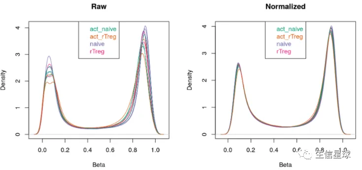
# visualise what the data looks like before and after normalisation
par(mfrow=c(1,2))
densityPlot(rgSet, sampGroups=targets$Sample_Group,main="Raw", legend=FALSE)
legend("top", legend = levels(factor(targets$Sample_Group)), 
       text.col=brewer.pal(8,"Dark2"))
densityPlot(getBeta(mSetSq), sampGroups=targets$Sample_Group,
            main="Normalized", legend=FALSE)
legend("top", legend = levels(factor(targets$Sample_Group)), 
       text.col=brewer.pal(8,"Dark2"))

接下来对得到的数据做个PCA看看

左边是4种不同的T-cell (naive, rTreg, act_naive, act_rTreg) 也是我们真心关注的；右边是3个不同的供体 (M28, M29, M30)，属于批次信息

par(mfrow=c(1,2))
plotMDS(getM(mSetSq), top=1000, gene.selection="common", 
        col=pal[factor(targets$Sample_Group)])
legend("top", legend=levels(factor(targets$Sample_Group)), text.col=pal,
       bg="white", cex=0.7)

plotMDS(getM(mSetSq), top=1000, gene.selection="common",  
        col=pal[factor(targets$Sample_Source)])
legend("top", legend=levels(factor(targets$Sample_Source)), text.col=pal,
       bg="white", cex=0.7)

右图就能清楚看到，PC1这么重要的位置，竟然让供体这个批次信息分的清清楚楚

因此，还需要继续优化这个批次信息

# 首先是过滤掉低质量探针（p值小于0.01）
detP <- detP[match(featureNames(mSetSq),rownames(detP)),] 
keep <- rowSums(detP < 0.01) == ncol(mSetSq) 
table(keep)
# keep
# FALSE   TRUE 
# 977 484535
mSetSqFlt <- mSetSq[keep,]
mSetSqFlt

# 由于我们这里都是男性，所以可以去掉性染色体上的探针。但是当数据的确存在性别差异的时候，也有特定的分析方法，见：http://bioconductor.org/packages/release/workflows/vignettes/methylationArrayAnalysis/inst/doc/methylationArrayAnalysis.html#differential-variability
keep <- !(featureNames(mSetSqFlt) %in% ann450k$Name[ann450k$chr %in% 
                                                        c("chrX","chrY")])
table(keep)
# keep
# FALSE   TRUE 
# 11608 472927
mSetSqFlt <- mSetSqFlt[keep,]

# remove probes with SNPs at CpG site
mSetSqFlt <- dropLociWithSnps(mSetSqFlt)
mSetSqFlt

# exclude cross reactive probes 
xReactiveProbes <- read.csv(file=paste(dataDirectory,
                                       "48639-non-specific-probes-Illumina450k.csv",
                                       sep="/"), stringsAsFactors=FALSE)
keep <- !(featureNames(mSetSqFlt) %in% xReactiveProbes$TargetID)
table(keep)
## keep
##  FALSE   TRUE 
##  27433 439918
mSetSqFlt <- mSetSqFlt[keep,] 
mSetSqFlt

再次画PCA图，看到这次供体信息从PC1中消失了，转为了次重点的PC2【因为横坐标PC1不能区分不同的供体，而纵坐标即PC2可以】：

再看看其他几个主成分，再一次确认了供体信息已经从PC1中移除，不过影响依旧存在。因此在后续的分析中，还是需要在model中设置individual这个factor

par(mfrow=c(1,3))
# Examine higher dimensions to look at other sources of variation
plotMDS(getM(mSetSqFlt), top=1000, gene.selection="common", 
        col=pal[factor(targets$Sample_Source)], dim=c(1,3))
legend("right", legend=levels(factor(targets$Sample_Source)), text.col=pal,
       cex=0.7, bg="white")

plotMDS(getM(mSetSqFlt), top=1000, gene.selection="common", 
        col=pal[factor(targets$Sample_Source)], dim=c(2,3))
legend("topright", legend=levels(factor(targets$Sample_Source)), text.col=pal,
       cex=0.7, bg="white")

plotMDS(getM(mSetSqFlt), top=1000, gene.selection="common", 
        col=pal[factor(targets$Sample_Source)], dim=c(3,4))
legend("right", legend=levels(factor(targets$Sample_Source)), text.col=pal,
       cex=0.7, bg="white")

计算M值与beta值

它们的区别是：

M-values have nicer statistical properties and are thus better for use in statistical analysis of methylation data 具有更好的统计意义，适合下面的差异分析
Beta values are easy to interpret and are thus better for displaying data. 更容易进行展示与解释
芯片上的每个CpG位点，都会计算两个值：methylated intensity (M表示)、unmethylated intensity (U表示)。它们的比值可以帮助判断每个CpG位点的甲基化水平。其中 Beta value = M/(M+U) ，而M = log2(M/U)

mVals <- getM(mSetSqFlt)
head(mVals[,1:5])
##              naive.1   rTreg.2 act_naive.3   naive.4 act_naive.5
## cg13869341  2.421276  2.515948    2.165745  2.286314    2.109441
## cg24669183  2.169414  2.235964    2.280734  1.632309    2.184435
## cg15560884  1.761176  1.577578    1.597503  1.777486    1.764999
## cg01014490 -3.504268 -3.825119   -5.384735 -4.537864   -4.296526
## cg17505339  3.082191  3.924931    4.163206  3.255373    3.654134
## cg11954957  1.546401  1.912204    1.727910  2.441267    1.618331

bVals <- getBeta(mSetSqFlt)
head(bVals[,1:5])
##               naive.1    rTreg.2 act_naive.3    naive.4 act_naive.5
## cg13869341 0.84267937 0.85118462   0.8177504 0.82987650  0.81186174
## cg24669183 0.81812908 0.82489238   0.8293297 0.75610281  0.81967323
## cg15560884 0.77219626 0.74903910   0.7516263 0.77417882  0.77266205
## cg01014490 0.08098986 0.06590459   0.0233755 0.04127262  0.04842397
## cg17505339 0.89439216 0.93822870   0.9471357 0.90520570  0.92641305
## cg11954957 0.74495496 0.79008516   0.7681146 0.84450764  0.75431167

甲基化信号值矩阵的差异分析

主要包括：

DMP：differential methylation probe（找位点），即一个一个的差异甲基化位点
DMR：differential methylation region（找区域），连续不断的差异化片段

首先是 Probe-wise differential methylation analysis

将使用limma的流程

# 将数据中的两个变量信息提出来
cellType <- factor(targets$Sample_Group)
individual <- factor(targets$Sample_Source) 

design <- model.matrix(~0+cellType+individual, data=targets)
colnames(design) <- c(levels(cellType),levels(individual)[-1])

注意这个design矩阵为什么要这么写：

# 来自：https://www.biostars.org/p/231771/ 
most people do with these experimental designs: 
~ 0 + DiseasePhenotype+ covariate + (1 | randomCovariate)
OR: y ~ 0 + effect1 + effect2 + (1 | effect 3)
# 这里DiseasePhenotype就是cellType，covariate就是individual

之前在：那些常用的limma操作中提过，limma需要的输入文件有：

表达矩阵（exprSet）（这个容易获得），转录组芯片数据可以通过exprs() ，常规的转录组可以通过read.csv()等导入
分组矩阵 (design) ：就是将表达矩阵的列（各个样本）分成几组（例如最简单的case - control，或者一些时间序列的样本day0, day1, day2 ...）【通过model.matrix()得到】
比较矩阵（contrast）：意思就是如何指定函数去进行组间比较【通过makeContrasts()得到】

# fit the linear model 
fit <- lmFit(mVals, design)
# create a contrast matrix for specific comparisons
contMatrix <- makeContrasts(naive-rTreg,
                            naive-act_naive,
                            rTreg-act_rTreg,
                            act_naive-act_rTreg,
                            levels=design)
# fit the contrasts
fit2 <- contrasts.fit(fit, contMatrix)
fit2 <- eBayes(fit2)
# look at the numbers of DM CpGs at FDR < 0.05
summary(decideTests(fit2))
##        naive - rTreg naive - act_naive rTreg - act_rTreg act_naive - act_rTreg
## Down            1618               400                 0                   559
## NotSig        436895            439291            439918                438440
## Up              1405               227                 0                   919

# 增加注释信息，其中topTable的参数coef=1表示保存为数据框
ann450kSub <- ann450k[match(rownames(mVals),ann450k$Name),
                      c(1:4,12:19,24:ncol(ann450k))]
DMPs <- topTable(fit2, num=Inf, coef=1, genelist=ann450kSub)
head(DMPs)

结果包含的列数很多，这里用两行来展示：

# plot the top 4 most significantly differentially methylated CpGs 
par(mfrow=c(2,2))
sapply(rownames(DMPs)[1:4], function(cpg){
    plotCpg(bVals, cpg=cpg, pheno=targets$Sample_Group, ylab = "Beta values")
})

然后是 Differential methylation analysis of regions

# using the dmrcate in the DMRcate package (Peters et al. 2015)
myAnnotation <- cpg.annotate(object = mVals, datatype = "array", what = "M", 
                             analysis.type = "differential", design = design, 
                             contrasts = TRUE, cont.matrix = contMatrix, 
                             coef = "naive - rTreg", arraytype = "450K")
DMRs <- dmrcate(myAnnotation, lambda=1000, C=2)
results.ranges <- extractRanges(DMRs)
results.ranges

可视化DMR

# set up the grouping variables and colours
groups <- pal[1:length(unique(targets$Sample_Group))]
names(groups) <- levels(factor(targets$Sample_Group))
cols <- groups[as.character(factor(targets$Sample_Group))]
# draw the plot for the top DMR
par(mfrow=c(1,1))
DMR.plot(ranges = results.ranges, dmr = 2, CpGs = bVals, phen.col = cols, 
         what = "Beta", arraytype = "450K", genome = "hg19")

Gene ontology testing

# Get the significant CpG sites at less than 5% FDR
sigCpGs <- DMPs$Name[DMPs$adj.P.Val<0.05]
# First 10 significant CpGs
sigCpGs[1:10]
##  [1] "cg07499259" "cg26992245" "cg09747445" "cg18808929" "cg25015733"
##  [6] "cg21179654" "cg26280976" "cg16943019" "cg10898310" "cg25130381"
length(sigCpGs) ## [1] 3023

# Get all the CpG sites used in the analysis to form the background
all <- DMPs$Name
# Total number of CpG sites tested
length(all) ## [1] 439918

# Top 10 GO categories
topGSA(gst, number=10)
##            ONTOLOGY                                        TERM    N  DE
## GO:0002376       BP                       immune system process 2895 383
## GO:0046649       BP                       lymphocyte activation  669 137
## GO:0042110       BP                           T cell activation  467 103
## GO:0002682       BP         regulation of immune system process 1480 219
## GO:0001775       BP                             cell activation 1378 206
## GO:0002520       BP                   immune system development  999 169
## GO:0048534       BP hematopoietic or lymphoid organ development  945 162
## GO:0022407       BP            regulation of cell-cell adhesion  431  93
## GO:0022409       BP   positive regulation of cell-cell adhesion  277  69
## GO:0007166       BP     cell surface receptor signaling pathway 2994 398
##                    P.DE          FDR
## GO:0002376 1.139863e-21 2.593075e-17
## GO:0046649 6.147656e-21 6.992652e-17
## GO:0042110 2.829736e-18 2.145788e-14
## GO:0002682 5.707044e-18 3.245738e-14
## GO:0001775 1.476431e-15 6.717465e-12
## GO:0002520 4.851443e-15 1.839424e-11
## GO:0048534 1.044579e-14 3.394733e-11
## GO:0022407 1.379734e-14 3.923445e-11
## GO:0022409 2.719337e-14 6.873578e-11
## GO:0007166 4.538082e-14 9.313273e-11

有用的资源

EWAS Data Hub：中国科学院北京基因组研究所国家基因组科学数据中心，开发了人类表观组关联分析数据库。EWAS Data Hub: a resource of DNA methylation array data and metadata. Nucleic Acids Res 2020. EWAS全称是：表观基因组广泛关联研究（Epigenome-wide Association Study，EWAS）https://bigd.big.ac.cn/ewas/datahub 包括了来自95,783个样本的DNA甲基化数据，数据主要来自GEO、TCGA、ArrayExpress和Encode数据库，采用有效的归一化方法来减轻不同数据集之间的批次效应，其中约91%是来自450K，来自血液样本的数据最多。Associations、Studies、Cohorts、Probe annotations、Trait to trait relationships都可以下载。
MEXPRESS：https://mexpress.be/ ，网页工具用于TCGA甲基化数据分析，结果包括临床信息、基因表达信息、拷贝数变化信息、甲基化位点变化信息、基因组长度、各个不同的转录本、cg位点的位置以及CpG岛的位置
表观遗传一些术语解释的不错：https://epigenie.com/key-epigenetic-players/

methylation