237- 和刘小泽一起跟着官网学maftools
刘小泽写于2021.3.10 官网在:http://bioconductor.org/packages/release/bioc/vignettes/maftools/inst/doc/maftools.html
0 简单了解MAF文件
关于MAF文件格式
TCGA测了33种癌症,每个GDC project,每个检测变异的流程都会得到一个MAF。
MAF全称是:Mutation Annotation Format (MAF) ,是tab分隔的文件,用于记录VCF中的 somatic 突变信息。它有两种类型:protected and somatic (or open-access)。
*protected.maf:一般VCF文件中会记录多个转录本变异信息,但是这个maf文件只会记录其中影响最大的那个*somatic.maf:又称Masked Somatic Mutation ,它去除了低质量以及潜在的germline变异,可以公开获取。
如何得到MAF文件
对于VCF文件或者一般的tab分隔的文件,比较简单的办法是利用: vcf2maf ,另外GATK也支持 funcotator可以生成MAF文件
如果使用ANNOVAR注释,可以利用
annovarToMaf进行转换
MAF需要的列
如果看官方说明文档:https://docs.gdc.cancer.gov/Data/File_Formats/MAF_Format/,会发现有上百列的信息,从最基本的基因组坐标,到更复杂的cosmic变异注释。
必须包含的列:Hugo_Symbol, Chromosome, Start_Position, End_Position, Reference_Allele, Tumor_Seq_Allele2, Variant_Classification, Variant_Type and Tumor_Sample_Barcode
推荐添加的其他列: VAF (Variant Allele Frequecy) , amino acid change information.
其中,有这么几列需要看下什么意思:
Reference_Allele: The plus strand reference allele at this position. Includes the deleted sequence for a deletion or “-” for an insertion
Variant_Classification: Translational effect of variant allele
Variant_Type: Type of mutation. TNP (tri-nucleotide polymorphism) is analogous to DNP (di-nucleotide polymorphism) but for three consecutive nucleotides. ONP (oligo-nucleotide polymorphism) is analogous to TNP but for consecutive runs of four or more (SNP, DNP, TNP, ONP, INS, DEL, or Consolidated)
Tumor_Sample_Barcode: Aliquot barcode for the tumor sample
下面👇将以TCGA LAML cohort 为例,来看看maftools的使用
1 准备工作
if (!require("BiocManager"))
    install.packages("BiocManager")
BiocManager::install("maftools")
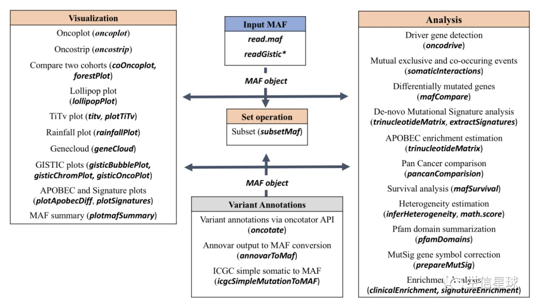
这个示意图解释的特别好: 把数据读取成maf对象,然后就可以画图或者分析
输入文件
(必须)MAF文件:可以是gz压缩的
(可选但建议)临床信息,并且与MAF中的sample对应
(可选)拷贝数信息:可以是GISTIC的结果或者自定义的tab文件(包含样本名称、基因名称以及拷贝数变异情况Amp或者Del)
2 读取文件
library(maftools)
suppressMessages(library(dplyr))
#(必须)TCGA LAML 的 MAF 文件
laml.maf = system.file('extdata', 'tcga_laml.maf.gz', package = 'maftools')
#(可选)临床信息
laml.clin = system.file('extdata', 'tcga_laml_annot.tsv', package = 'maftools')

laml = read.maf(maf = laml.maf, clinicalData = laml.clin)
## -Reading
## -Validating
## -Silent variants: 475
## -Summarizing
## -Processing clinical data
## -Finished in 0.290s elapsed (0.243s cpu)
看看读取的对象中包含什么
laml
## An object of class  MAF
##                    ID          summary  Mean Median
##  1:        NCBI_Build               37    NA     NA
##  2:            Center genome.wustl.edu    NA     NA
##  3:           Samples              193    NA     NA
##  4:            nGenes             1241    NA     NA
##  5:   Frame_Shift_Del               52 0.269      0
##  6:   Frame_Shift_Ins               91 0.472      0
##  7:      In_Frame_Del               10 0.052      0
##  8:      In_Frame_Ins               42 0.218      0
##  9: Missense_Mutation             1342 6.953      7
## 10: Nonsense_Mutation              103 0.534      0
## 11:       Splice_Site               92 0.477      0
## 12:             total             1732 8.974      9
#Shows sample summry.
getSampleSummary(laml)
##      Tumor_Sample_Barcode Frame_Shift_Del
##   1:         TCGA-AB-3009               0
##   2:         TCGA-AB-2807               1
##   3:         TCGA-AB-2959               0
##   4:         TCGA-AB-3002               0
##   5:         TCGA-AB-2849               0
##  ---
## 189:         TCGA-AB-2942               0
## 190:         TCGA-AB-2946               0
## 191:         TCGA-AB-2954               0
## 192:         TCGA-AB-2982               0
## 193:         TCGA-AB-2903               0
##      Frame_Shift_Ins In_Frame_Del In_Frame_Ins
##   1:               5            0            1
##   2:               0            1            0
##   3:               0            0            0
##   4:               0            0            0
##   5:               1            0            0
##  ---
## 189:               0            0            1
## 190:               0            0            0
## 191:               0            0            0
## 192:               0            0            0
## 193:               0            0            0
##      Missense_Mutation Nonsense_Mutation Splice_Site
##   1:                25                 2           1
##   2:                16                 3           4
##   3:                22                 0           1
##   4:                15                 1           5
##   5:                16                 1           2
##  ---
## 189:                 0                 0           0
## 190:                 1                 0           0
## 191:                 1                 0           0
## 192:                 1                 0           0
## 193:                 0                 0           0
##      total
##   1:    34
##   2:    25
##   3:    23
##   4:    21
##   5:    20
##  ---
## 189:     1
## 190:     1
## 191:     1
## 192:     1
## 193:     0
#Shows gene summary.
getGeneSummary(laml)
##       Hugo_Symbol Frame_Shift_Del Frame_Shift_Ins
##    1:        FLT3               0               0
##    2:      DNMT3A               4               0
##    3:        NPM1               0              33
##    4:        IDH2               0               0
##    5:        IDH1               0               0
##   ---
## 1237:      ZNF689               0               0
## 1238:      ZNF75D               0               0
## 1239:      ZNF827               1               0
## 1240:       ZNF99               0               0
## 1241:        ZPBP               0               0
##       In_Frame_Del In_Frame_Ins Missense_Mutation
##    1:            1           33                15
##    2:            0            0                39
##    3:            0            0                 1
##    4:            0            0                20
##    5:            0            0                18
##   ---
## 1237:            0            0                 1
## 1238:            0            0                 1
## 1239:            0            0                 0
## 1240:            0            0                 1
## 1241:            0            0                 1
##       Nonsense_Mutation Splice_Site total MutatedSamples
##    1:                 0           3    52             52
##    2:                 5           6    54             48
##    3:                 0           0    34             33
##    4:                 0           0    20             20
##    5:                 0           0    18             18
##   ---
## 1237:                 0           0     1              1
## 1238:                 0           0     1              1
## 1239:                 0           0     1              1
## 1240:                 0           0     1              1
## 1241:                 0           0     1              1
##       AlteredSamples
##    1:             52
##    2:             48
##    3:             33
##    4:             20
##    5:             18
##   ---
## 1237:              1
## 1238:              1
## 1239:              1
## 1240:              1
## 1241:              1
#shows clinical data associated with samples
getClinicalData(laml)
##      Tumor_Sample_Barcode FAB_classification
##   1:         TCGA-AB-2802                 M4
##   2:         TCGA-AB-2803                 M3
##   3:         TCGA-AB-2804                 M3
##   4:         TCGA-AB-2805                 M0
##   5:         TCGA-AB-2806                 M1
##  ---
## 189:         TCGA-AB-3007                 M3
## 190:         TCGA-AB-3008                 M1
## 191:         TCGA-AB-3009                 M4
## 192:         TCGA-AB-3011                 M1
## 193:         TCGA-AB-3012                 M3
##      days_to_last_followup Overall_Survival_Status
##   1:                   365                       1
##   2:                   792                       1
##   3:                  2557                       0
##   4:                   577                       1
##   5:                   945                       1
##  ---
## 189:                  1581                       0
## 190:                   822                       1
## 191:                   577                       1
## 192:                  1885                       0
## 193:                  1887                       0
#Shows all fields in MAF
getFields(laml)
##  [1] "Hugo_Symbol"            "Entrez_Gene_Id"
##  [3] "Center"                 "NCBI_Build"
##  [5] "Chromosome"             "Start_Position"
##  [7] "End_Position"           "Strand"
##  [9] "Variant_Classification" "Variant_Type"
## [11] "Reference_Allele"       "Tumor_Seq_Allele1"
## [13] "Tumor_Seq_Allele2"      "Tumor_Sample_Barcode"
## [15] "Protein_Change"         "i_TumorVAF_WU"
## [17] "i_transcript_name"
#Writes maf summary to an output file with basename laml.
write.mafSummary(maf = laml, basename = 'laml')
3 可视化
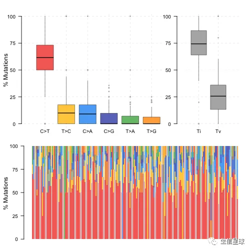
3.1 MAF概览图 | Summary
plotmafSummary(maf = laml, rmOutlier = TRUE, addStat = 'median', dashboard = TRUE, titvRaw = FALSE)

# 下面看看它们各自利用的数据
# 图A
apply(laml@variant.classification.summary[,2:8], 2, sum)
##   Frame_Shift_Del   Frame_Shift_Ins      In_Frame_Del
##                52                91                10
##      In_Frame_Ins Missense_Mutation Nonsense_Mutation
##                42              1342               103
##       Splice_Site
##                92
# 图B
apply(laml@variant.type.summary[,2:4], 2, sum)
##  DEL  INS  SNP
##   64  141 1527
# 图D
head(laml@variants.per.sample)
##    Tumor_Sample_Barcode Variants
## 1:         TCGA-AB-3009       34
## 2:         TCGA-AB-2807       25
## 3:         TCGA-AB-2959       23
## 4:         TCGA-AB-3002       21
## 5:         TCGA-AB-2923       20
## 6:         TCGA-AB-2972       20
# 图E和图A类似,只是把barplot换成了boxplot
# 图F
laml@gene.summary %>% arrange(desc(total))
##       Hugo_Symbol Frame_Shift_Del Frame_Shift_Ins
##    1:      DNMT3A               4               0
##    2:        FLT3               0               0
##    3:        NPM1               0              33
##    4:        TET2              10               4
##    5:        IDH2               0               0
##   ---
## 1237:      ZNF689               0               0
## 1238:      ZNF75D               0               0
## 1239:      ZNF827               1               0
## 1240:       ZNF99               0               0
## 1241:        ZPBP               0               0
##       In_Frame_Del In_Frame_Ins Missense_Mutation
##    1:            0            0                39
##    2:            1           33                15
##    3:            0            0                 1
##    4:            0            0                 4
##    5:            0            0                20
##   ---
## 1237:            0            0                 1
## 1238:            0            0                 1
## 1239:            0            0                 0
## 1240:            0            0                 1
## 1241:            0            0                 1
##       Nonsense_Mutation Splice_Site total MutatedSamples
##    1:                 5           6    54             48
##    2:                 0           3    52             52
##    3:                 0           0    34             33
##    4:                 8           1    27             17
##    5:                 0           0    20             20
##   ---
## 1237:                 0           0     1              1
## 1238:                 0           0     1              1
## 1239:                 0           0     1              1
## 1240:                 0           0     1              1
## 1241:                 0           0     1              1
##       AlteredSamples
##    1:             48
##    2:             52
##    3:             33
##    4:             17
##    5:             20
##   ---
## 1237:              1
## 1238:              1
## 1239:              1
## 1240:              1
## 1241:              1
至于图3:
# https://rdrr.io/bioc/maftools/src/R/titv.R
maf=laml
mafDat = subsetMaf(maf = maf, query = "Variant_Type == 'SNP'", mafObj = FALSE, includeSyn = T, fields = "Variant_Type")
mafDat$con = paste(mafDat[,Reference_Allele], mafDat[,Tumor_Seq_Allele2], sep = '>')

conv = c("T>C", "T>C", "C>T", "C>T", "T>A", "T>A", "T>G", "T>G", "C>A", "C>A", "C>G", "C>G")
names(conv) = c('A>G', 'T>C', 'C>T', 'G>A', 'A>T', 'T>A', 'A>C', 'T>G', 'C>A', 'G>T', 'C>G', 'G>C')
mafDat = mafDat[con %in% names(conv)]
mafDat$con.class = conv[as.character(mafDat$con)]
table(mafDat$con.class )
##
##  C>A  C>G  C>T  T>A  T>C  T>G
##  235  139 1235   89  236   68
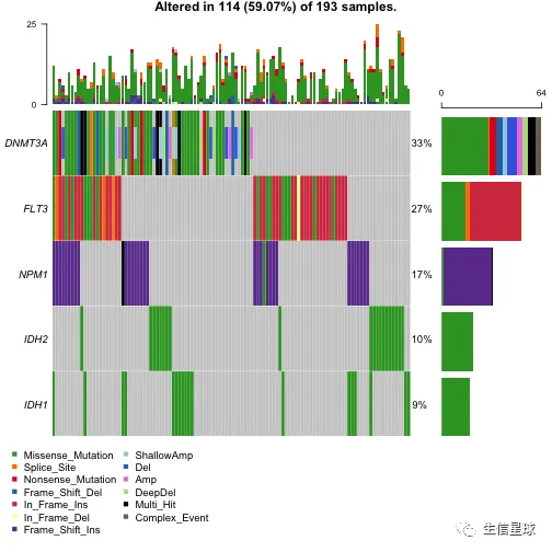
3.2 突变全景图/瀑布图 | Oncoplots
#oncoplot for top ten mutated genes.
oncoplot(maf = laml, top = 10)
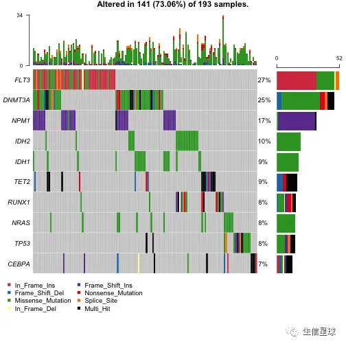
- 默认绘制top10基因,当然可以设置参数
genes只展示某几个感兴趣的基因 - 注意其中有一个legend叫做:”Multi Hit“,它指的是某个基因在一个样本中突变次数超过1
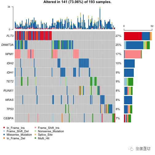
给图例换个颜色
#One can use any colors, here in this example color palette from RColorBrewer package is used
vc_cols = RColorBrewer::brewer.pal(n = 8, name = 'Paired')
names(vc_cols) = c(
  'Frame_Shift_Del',
  'Missense_Mutation',
  'Nonsense_Mutation',
  'Multi_Hit',
  'Frame_Shift_Ins',
  'In_Frame_Ins',
  'Splice_Site',
  'In_Frame_Del'
)

print(vc_cols)
##   Frame_Shift_Del Missense_Mutation Nonsense_Mutation
##         "#A6CEE3"         "#1F78B4"         "#B2DF8A"
##         Multi_Hit   Frame_Shift_Ins      In_Frame_Ins
##         "#33A02C"         "#FB9A99"         "#E31A1C"
##       Splice_Site      In_Frame_Del
##         "#FDBF6F"         "#FF7F00"
oncoplot(maf = laml, colors = vc_cols, top = 10)
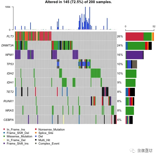
如果要包含拷贝数的数据
使用GISTIC结果
GISTIC会得到许多结果文件,我们需要的是:all_lesions.conf_XX.txt, amp_genes.conf_XX.txt, del_genes.conf_XX.txt, scores.gistic,其中XX指的是可信度(confidence level)
#GISTIC results LAML
all.lesions =
  system.file("extdata", "all_lesions.conf_99.txt", package = "maftools")
amp.genes =
  system.file("extdata", "amp_genes.conf_99.txt", package = "maftools")
del.genes =
  system.file("extdata", "del_genes.conf_99.txt", package = "maftools")
scores.gis =
  system.file("extdata", "scores.gistic", package = "maftools")

#Read GISTIC results along with MAF
laml.plus.gistic = read.maf(
  maf = laml.maf,
  gisticAllLesionsFile = all.lesions,
  gisticAmpGenesFile = amp.genes,
  gisticDelGenesFile = del.genes,
  gisticScoresFile = scores.gis,
  isTCGA = TRUE,
  verbose = FALSE,
  clinicalData = laml.clin
)
oncoplot(maf = laml.plus.gistic, top = 10)
使用自定义的结果
比如这里给DNMT3A基因创建一个20个样本的拷贝数变异数据
set.seed(seed = 1024)
barcodes = as.character(getSampleSummary(x = laml)[,Tumor_Sample_Barcode])
#Random 20 samples
dummy.samples = sample(x = barcodes,
                       size = 20,
                       replace = FALSE)

#Genarate random CN status for above samples
cn.status = sample(
  x = c('ShallowAmp', 'DeepDel', 'Del', 'Amp'),
  size = length(dummy.samples),
  replace = TRUE
)

custom.cn.data = data.frame(
  Gene = "DNMT3A",
  Sample_name = dummy.samples,
  CN = cn.status,
  stringsAsFactors = FALSE
)
head(custom.cn.data)
##     Gene  Sample_name         CN
## 1 DNMT3A TCGA-AB-2898 ShallowAmp
## 2 DNMT3A TCGA-AB-2879        Del
## 3 DNMT3A TCGA-AB-2920        Amp
## 4 DNMT3A TCGA-AB-2866        Del
## 5 DNMT3A TCGA-AB-2892        Del
## 6 DNMT3A TCGA-AB-2863 ShallowAmp
laml.plus.cn = read.maf(maf = laml.maf,
                        cnTable = custom.cn.data,
                        verbose = FALSE)
oncoplot(maf = laml.plus.cn, top = 5)
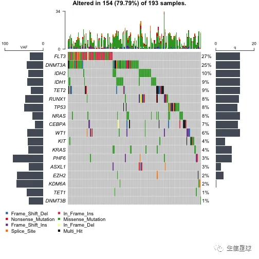
添加左右两侧的barplot
可以使用leftBarData, rightBarData, topBarData
#Selected AML driver genes
aml_genes = c("TP53", "WT1", "PHF6", "DNMT3A", "DNMT3B", "TET1", "TET2", "IDH1", "IDH2", "FLT3", "KIT", "KRAS", "NRAS", "RUNX1", "CEBPA", "ASXL1", "EZH2", "KDM6A")

#Variant allele frequcnies (Left bar plot)
aml_genes_vaf = subsetMaf(maf = laml, genes = aml_genes, fields = "i_TumorVAF_WU", mafObj = FALSE)[,mean(i_TumorVAF_WU, na.rm = TRUE), Hugo_Symbol]
colnames(aml_genes_vaf)[2] = "VAF"
head(aml_genes_vaf)
##    Hugo_Symbol      VAF
## 1:       ASXL1 37.11250
## 2:       CEBPA 22.00235
## 3:      DNMT3A 43.51556
## 4:      DNMT3B 37.14000
## 5:        EZH2 68.88500
## 6:        FLT3 34.60294
#MutSig results (Right bar plot)
laml.mutsig = system.file("extdata", "LAML_sig_genes.txt.gz", package = "maftools")
laml.mutsig = data.table::fread(input = laml.mutsig)[,.(gene, q)]
laml.mutsig[,q := -log10(q)] #transoform to log10
head(laml.mutsig)
##      gene        q
## 1:   FLT3 12.64176
## 2: DNMT3A 12.64176
## 3:   NPM1 12.64176
## 4:   IDH2 12.64176
## 5:   IDH1 12.64176
## 6:   TET2 12.64176
# 如果这里画图报错,说找不到参数,那么可能就需要更新到R 版本4以上的maftools包了
oncoplot(
  maf = laml,
  genes = aml_genes,
  leftBarData = aml_genes_vaf,
  leftBarLims = c(0, 100),
  rightBarData = laml.mutsig,
  rightBarLims = c(0, 20)
)
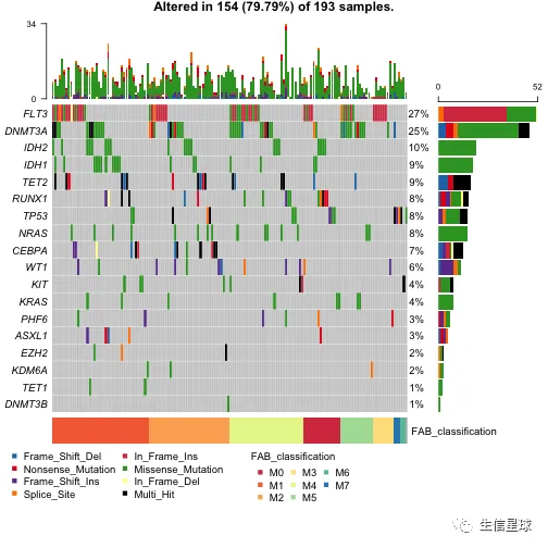
添加临床信息
getClinicalData(x = laml)
##      Tumor_Sample_Barcode FAB_classification
##   1:         TCGA-AB-2802                 M4
##   2:         TCGA-AB-2803                 M3
##   3:         TCGA-AB-2804                 M3
##   4:         TCGA-AB-2805                 M0
##   5:         TCGA-AB-2806                 M1
##  ---
## 189:         TCGA-AB-3007                 M3
## 190:         TCGA-AB-3008                 M1
## 191:         TCGA-AB-3009                 M4
## 192:         TCGA-AB-3011                 M1
## 193:         TCGA-AB-3012                 M3
##      days_to_last_followup Overall_Survival_Status
##   1:                   365                       1
##   2:                   792                       1
##   3:                  2557                       0
##   4:                   577                       1
##   5:                   945                       1
##  ---
## 189:                  1581                       0
## 190:                   822                       1
## 191:                   577                       1
## 192:                  1885                       0
## 193:                  1887                       0
oncoplot(maf = laml, genes = aml_genes, clinicalFeatures = 'FAB_classification')
# 还可以自定义颜色
fabcolors = RColorBrewer::brewer.pal(n = 8,name = 'Spectral')
names(fabcolors) = c("M0", "M1", "M2", "M3", "M4", "M5", "M6", "M7")
fabcolors = list(FAB_classification = fabcolors)

print(fabcolors)
## $FAB_classification
##        M0        M1        M2        M3        M4
## "#D53E4F" "#F46D43" "#FDAE61" "#FEE08B" "#E6F598"
##        M5        M6        M7
## "#ABDDA4" "#66C2A5" "#3288BD"
oncoplot(
  maf = laml, genes = aml_genes,
  clinicalFeatures = 'FAB_classification',
  sortByAnnotation = TRUE,
  annotationColor = fabcolors
)
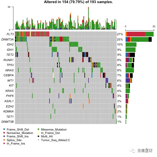
突出显示某些样本
比如:突出显示alt allele is C的样本
# 看看有哪些列
getFields(x = laml)
##  [1] "Hugo_Symbol"            "Entrez_Gene_Id"
##  [3] "Center"                 "NCBI_Build"
##  [5] "Chromosome"             "Start_Position"
##  [7] "End_Position"           "Strand"
##  [9] "Variant_Classification" "Variant_Type"
## [11] "Reference_Allele"       "Tumor_Seq_Allele1"
## [13] "Tumor_Seq_Allele2"      "Tumor_Sample_Barcode"
## [15] "Protein_Change"         "i_TumorVAF_WU"
## [17] "i_transcript_name"
# 然后使用参数additionalFeature
oncoplot(maf = laml, genes = aml_genes,
         additionalFeature = c("Tumor_Seq_Allele2", "C"))
各种组合
oncoplot(
  maf = laml.plus.gistic,
  draw_titv = TRUE,
  clinicalFeatures = c('FAB_classification', 'Overall_Survival_Status'),
  sortByAnnotation = TRUE,
  additionalFeature = c("Tumor_Seq_Allele2", "C"),
  leftBarData = aml_genes_vaf,
  leftBarLims = c(0, 100),
  rightBarData = laml.mutsig[,.(gene, q)],
)
3.3 转换和颠换 | Transition and Transversions
名词解释:http://www.mun.ca/biology/scarr/Transitions_vs_Transversions.html
使用titv函数,画出箱线图,显示六种不同转换的总体分布,还有堆积条形图显示每个样本中的转换比例。
laml.titv = titv(maf = laml, plot = FALSE, useSyn = TRUE)
plotTiTv(res = laml.titv)
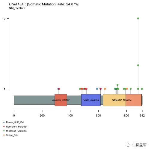
3.4 氨基酸突变热点 | Lollipop plots
许多癌基因,某些位点比其他位点更容易突变,变异频率更高,这些位置被认为是突变热点(hot-spots)。
使用函数lollipopPlot,需要我们在maf中给出氨基酸改变的信息。它默认寻找名字为"AAChange"的列,如果找不到,会给出一个warning信息,并且列出所有的列名。然后通过参数AACol进行指定。另外,它默认使用最长的gene isoform
lollipopPlot(maf = laml, gene = 'DNMT3A', AACol = 'Protein_Change', showMutationRate = TRUE)
##      HGNC refseq.ID protein.ID aa.length
## 1: DNMT3A NM_175629  NP_783328       912
## 2: DNMT3A NM_022552  NP_072046       912
## 3: DNMT3A NM_153759  NP_715640       723
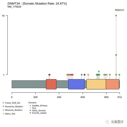
可以只画某个位点(如果设置labelPos=='all',就会画所有的位点)
laml@data$Protein_Change[grepl('882',laml@data$Protein_Change)]
##  [1] "p.R882C" "p.R882H" "p.R882C" "p.R882H" "p.R882P"
##  [6] "p.R882H" "p.R882H" "p.R882H" "p.R882H" "p.R882H"
## [11] "p.R882H" "p.R882H" "p.R882H" "p.R882H" "p.R882C"
## [16] "p.R882C" "p.R882H" "p.R882C" "p.R882H" "p.R882H"
## [21] "p.R882H" "p.R882H" "p.R882H" "p.R882C" "p.R882H"
## [26] "p.R882C" "p.R882H"
lollipopPlot(maf = laml, gene = 'DNMT3A', showDomainLabel = FALSE, labelPos = 882)
##      HGNC refseq.ID protein.ID aa.length
## 1: DNMT3A NM_175629  NP_783328       912
## 2: DNMT3A NM_022552  NP_072046       912
## 3: DNMT3A NM_153759  NP_715640       723
3.5 体细胞超突变 | Rainfall plots (RP)
名词解释:Somatic hypermutation (or SHM) 体细胞超突变, 指让基因组以背景突变率的至少十万倍到百万倍的高频率发生突变的细胞机制,主要形式是点突变(单碱基取代),偶见碱基插入或缺失。免疫系统的B细胞和多种癌细胞都可以使用此机制。
brca <- system.file("extdata", "brca.maf.gz", package = "maftools")
brca = read.maf(maf = brca, verbose = FALSE)

# If detectChangePoints is set to TRUE, rainfall plot also highlights regions where potential changes in inter-event distances are located.
rainfallPlot(maf = brca, detectChangePoints = TRUE, pointSize = 0.4)
##    Chromosome Start_Position End_Position nMuts
## 1:          8       98129348     98133560     7
## 2:          8       98398549     98403536     9
## 3:          8       98453076     98456466     9
## 4:          8      124090377    124096810    22
## 5:         12       97436055     97439705     7
## 6:         17       29332072     29336153     8
##    Avg_intermutation_dist Size Tumor_Sample_Barcode C>G
## 1:               702.0000 4212         TCGA-A8-A08B   4
## 2:               623.3750 4987         TCGA-A8-A08B   1
## 3:               423.7500 3390         TCGA-A8-A08B   1
## 4:               306.3333 6433         TCGA-A8-A08B   1
## 5:               608.3333 3650         TCGA-A8-A08B   4
## 6:               583.0000 4081         TCGA-A8-A08B   4
##    C>T
## 1:   3
## 2:   8
## 3:   8
## 4:  21
## 5:   3
## 6:   4
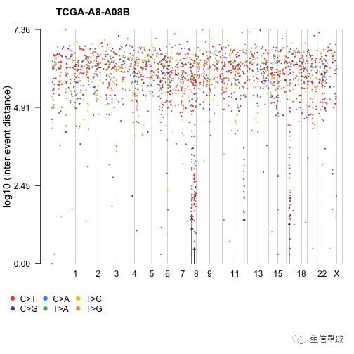
图片会输出Kataegis的具体信息,并在图中用黑色箭头进行标记。
“Kataegis”are defined as those genomic segments containing six or more consecutive mutations with an average inter-mutation distance of less than or equal to 1,00 bp 即:包含至少6个连续突变的基因组区段,并且平均突变间距离不大于100bp
关于这个图的更多解释,有人写了篇paper:https://bmcbioinformatics.biomedcentral.com/articles/10.1186/s12859-017-1679-8
The plot is mostly used for illustrating the distribution of somatic cancer mutations along a reference genome, typically aiming to identify mutation hotspots. The x-coordinate shows the genomic position of the mutation, while the y-coordinate represents the base pair distance between consecutive mutations on a logarithmic scale.
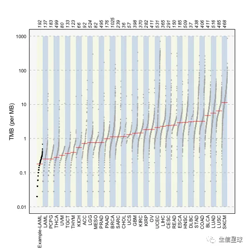
3.6 样本肿瘤突变负荷 | TMB
TMB在许多癌症与预后相关,maftools也内置了33个TCGA癌症队列的突变数据
# 看源代码https://github.com/PoisonAlien/maftools/blob/master/R/tcgacompare.R,它使用的是mc3.v0.2.8.PUBLIC.maf.gz(https://api.gdc.cancer.gov/data/1c8cfe5f-e52d-41ba-94da-f15ea1337efc, 35.8 MB)

# TCGA的样本
tcga.cohort = system.file('extdata', 'tcga_cohort.txt.gz', package = 'maftools')
tcga.cohort = data.table::fread(file = tcga.cohort, sep = '\t', stringsAsFactors = FALSE)
head(tcga.cohort)
##    cohort         Tumor_Sample_Barcode total
## 1:    ACC TCGA-OR-A5KB-01A-11D-A30A-10  1803
## 2:    ACC TCGA-PK-A5HB-01A-11D-A29I-10   962
## 3:    ACC TCGA-OR-A5JA-01A-11D-A29I-10   464
## 4:    ACC TCGA-OR-A5LJ-01A-11D-A29I-10   395
## 5:    ACC TCGA-OR-A5J5-01A-11D-A29I-10   349
## 6:    ACC TCGA-OR-A5JB-01A-11D-A29I-10   277
##                       site
## 1: Adrenal Gland Carcinoma
## 2: Adrenal Gland Carcinoma
## 3: Adrenal Gland Carcinoma
## 4: Adrenal Gland Carcinoma
## 5: Adrenal Gland Carcinoma
## 6: Adrenal Gland Carcinoma
# 我们的样本
dim(laml@variants.per.sample)
## [1] 192 2
head(laml@variants.per.sample)
##    Tumor_Sample_Barcode Variants
## 1:         TCGA-AB-3009       34
## 2:         TCGA-AB-2807       25
## 3:         TCGA-AB-2959       23
## 4:         TCGA-AB-3002       21
## 5:         TCGA-AB-2923       20
## 6:         TCGA-AB-2972       20
laml.mutload = tcgaCompare(maf = laml, cohortName = 'Example-LAML', logscale = TRUE, capture_size = 50)
3.7 变异等位基因频率 | Variant Allele Frequencies (VAF)
可以看:https://byteofbio.com/archives/7.html
VAF的全称是Variant Allele Frequency(变异等位基因频率)或Variant Allele Fraction(变异等位基因分数),指的是在基因组某个位点支持alternate/mutant allele的reads覆盖深度占这个位点总reads覆盖深度的比例。
在VCF文件中,DP表示Total Depth,AD表示Allele Depth
这里的VAF=AD/DP
plotVafhelps to estimate clonal status of top mutated genes (clonal genes usually have mean allele frequency around ~50% assuming pure sample)
plotVaf(maf = laml, vafCol = 'i_TumorVAF_WU')
4 处理拷贝数数据
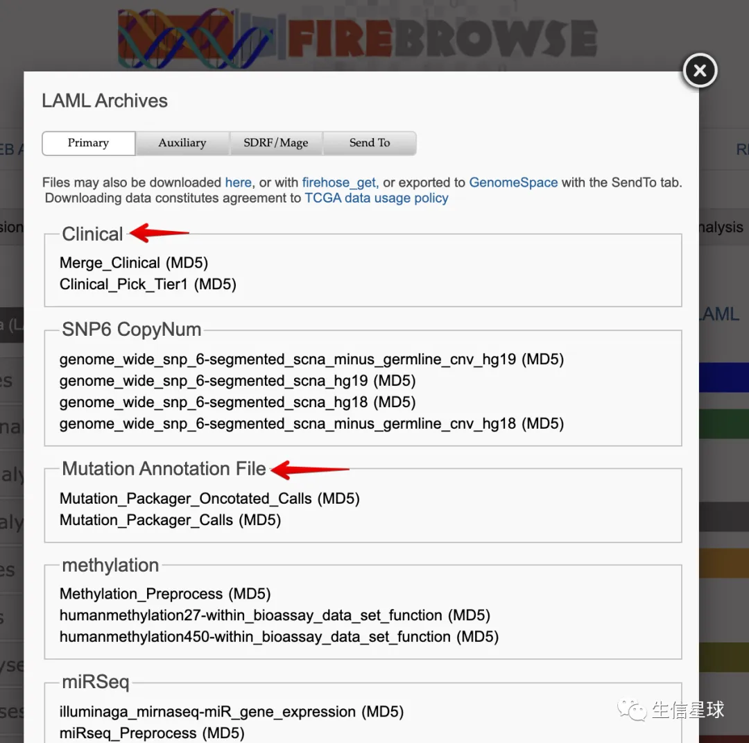
还是利用GISTIC生成的4个文件:all_lesions.conf_XX.txt, amp_genes.conf_XX.txt, del_genes.conf_XX.txt, scores.gistic 从Firehose也能下载,但是版本就会比较老(2016_01_18),而且用的是hg19,而TCGA目前都是基于hg38
如果要从firehose下载
以TCGA-LAML为例: 链接版: http://gdac.broadinstitute.org/runs/stddata__2016_01_28/data/LAML/20160128/
界面版: http://firebrowse.org/?cohort=LAML&download_dialog=true 然后这么操作:
不过还需要注意:基于hg19的firehose的基因组坐标,与官方TCGA的hg38坐标不一致,所以如果CNV数据从firehose下载,那么临床信息与MAF文件也需要从firehose下载
读取数据
# R包自带
all.lesions <- system.file("extdata", "all_lesions.conf_99.txt", package = "maftools")
amp.genes <- system.file("extdata", "amp_genes.conf_99.txt", package = "maftools")
del.genes <- system.file("extdata", "del_genes.conf_99.txt", package = "maftools")
scores.gis <- system.file("extdata", "scores.gistic", package = "maftools")

laml.gistic = readGistic(gisticAllLesionsFile = all.lesions,
                         gisticAmpGenesFile = amp.genes,
                         gisticDelGenesFile = del.genes,
                         gisticScoresFile = scores.gis,
                         isTCGA = TRUE)
## -Processing Gistic files..
## --Processing amp_genes.conf_99.txt
## --Processing del_genes.conf_99.txt
## --Processing scores.gistic
## --Summarizing by samples
laml.gistic
## An object of class  GISTIC
##           ID summary
## 1:   Samples     191
## 2:    nGenes    2622
## 3: cytoBands      16
## 4:       Amp     388
## 5:       Del   26481
## 6:     total   26869
# 自己firehose下载
my.all.lesions <- 'gdac.broadinstitute.org_LAML-TB.CopyNumber_Gistic2.Level_4.2016012800.0.0/all_lesions.conf_99.txt'
my.amp.genes <- 'gdac.broadinstitute.org_LAML-TB.CopyNumber_Gistic2.Level_4.2016012800.0.0/amp_genes.conf_99.txt'
my.del.genes <- 'gdac.broadinstitute.org_LAML-TB.CopyNumber_Gistic2.Level_4.2016012800.0.0/del_genes.conf_99.txt'
my.scores.gis <- 'gdac.broadinstitute.org_LAML-TB.CopyNumber_Gistic2.Level_4.2016012800.0.0/scores.gistic'

my.laml.gistic = readGistic(gisticAllLesionsFile = my.all.lesions,
                         gisticAmpGenesFile = my.amp.genes,
                         gisticDelGenesFile = my.del.genes,
                         gisticScoresFile = my.scores.gis,
                         isTCGA = TRUE)
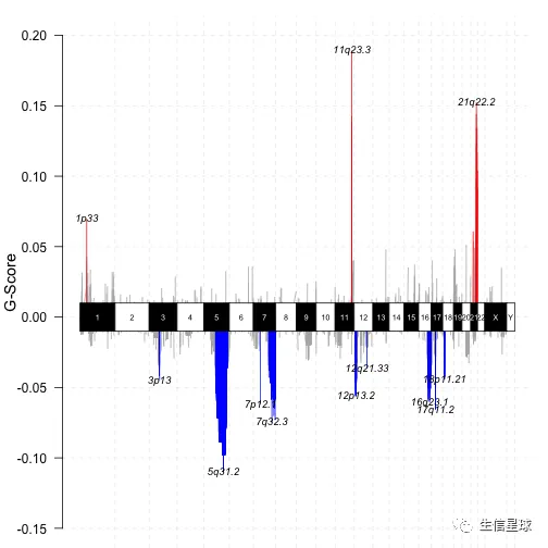
可视化
# genome plot
gisticChromPlot(gistic = laml.gistic, markBands = "all")
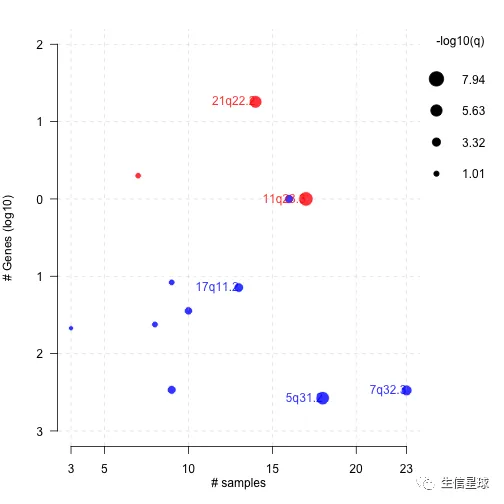
#  Bubble plot
gisticBubblePlot(gistic = laml.gistic)
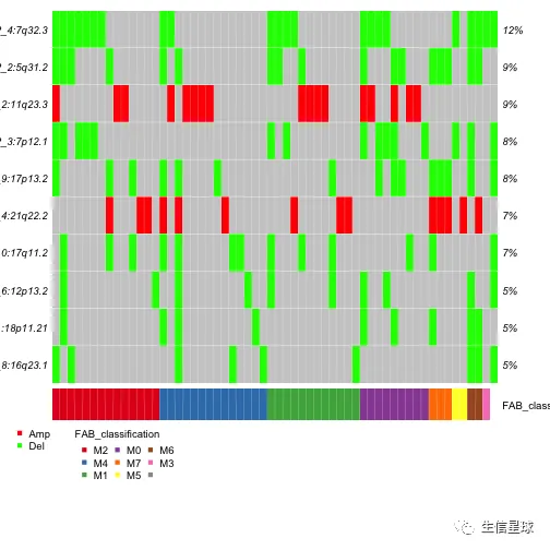
# oncoplot
# 图中显示:7q deletions 在M4亚型中是缺乏的,但在其他几个亚型中存在
laml.maf = system.file('extdata', 'tcga_laml.maf.gz', package = 'maftools')
laml.clin = system.file('extdata', 'tcga_laml_annot.tsv', package = 'maftools')
laml = read.maf(maf = laml.maf, clinicalData = laml.clin)
## -Reading
## -Validating
## -Silent variants: 475
## -Summarizing
## -Processing clinical data
## -Finished in 0.256s elapsed (0.231s cpu)
gisticOncoPlot(gistic = laml.gistic,
               clinicalData = getClinicalData(x = laml),
               clinicalFeatures = 'FAB_classification',
               sortByAnnotation = TRUE, top = 10)
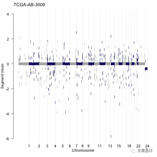
除了输出GISTIC的结果,还可以输出DNAcopy的segment结果
tcga.ab.009.seg <- system.file("extdata", "TCGA.AB.3009.hg19.seg.txt", package = "maftools")
plotCBSsegments(cbsFile = tcga.ab.009.seg)
## NULL
5 可以做的分析
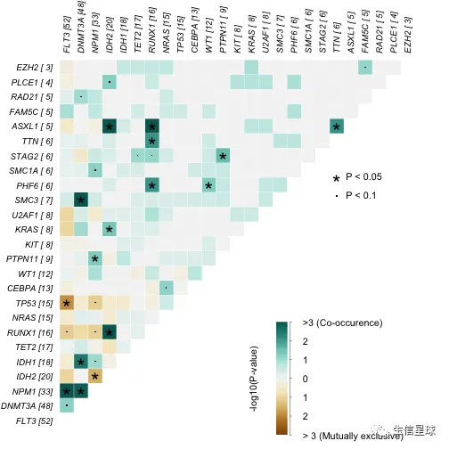
5.1 检测互斥或共存的突变 | somaticInteractions
它是选队列中突变最多的top基因(设定参数top=10),或者指定基因(设定参数genes=c()),进行pair-wise Fisher’s Exact test
检测共突变的意义是区别于单基因突变,治疗方法和后期用药都会存在不同。结果中绿色是倾向共存的突变基因;黄色是倾向互斥,颜色深浅表示显著性
#exclusive/co-occurance event analysis on top 10 mutated genes.
somaticInteractions(maf = laml, top = 25, pvalue = c(0.05, 0.1))
##      gene1  gene2       pValue oddsRatio  00 11 01 10
##   1: ASXL1  RUNX1 0.0001541586 55.215541 176  4 12  1
##   2:  IDH2  RUNX1 0.0002809928  9.590877 164  7  9 13
##   3:  IDH2  ASXL1 0.0004030636 41.077327 172  4  1 16
##   4:  FLT3   NPM1 0.0009929836  3.763161 125 17 16 35
##   5:  SMC3 DNMT3A 0.0010451985 20.177713 144  6 42  1
##  ---
## 296: PLCE1  ASXL1 1.0000000000  0.000000 184  0  5  4
## 297: RAD21  FAM5C 1.0000000000  0.000000 183  0  5  5
## 298: PLCE1  FAM5C 1.0000000000  0.000000 184  0  5  4
## 299: PLCE1  RAD21 1.0000000000  0.000000 184  0  5  4
## 300:  EZH2  PLCE1 1.0000000000  0.000000 186  0  4  3
##                   Event         pair event_ratio
##   1:       Co_Occurence ASXL1, RUNX1        4/13
##   2:       Co_Occurence  IDH2, RUNX1        7/22
##   3:       Co_Occurence  ASXL1, IDH2        4/17
##   4:       Co_Occurence   FLT3, NPM1       17/51
##   5:       Co_Occurence DNMT3A, SMC3        6/43
##  ---
## 296: Mutually_Exclusive ASXL1, PLCE1         0/9
## 297: Mutually_Exclusive FAM5C, RAD21        0/10
## 298: Mutually_Exclusive FAM5C, PLCE1         0/9
## 299: Mutually_Exclusive PLCE1, RAD21         0/9
## 300: Mutually_Exclusive  EZH2, PLCE1         0/7
5.2 预测癌症驱动基因 | oncodrive
函数oncodrive基于
oncodriveCLUST 算法,从MAF文件中预测驱动基因。它是根据:癌症驱动基因的突变一般富集在某些特定位点(即hot-spots),然后利用这些位点去鉴定基因。
laml.sig = oncodrive(maf = laml, AACol = 'Protein_Change', minMut = 5, pvalMethod = 'zscore')
head(laml.sig)
##    Hugo_Symbol Frame_Shift_Del Frame_Shift_Ins
## 1:        IDH1               0               0
## 2:        IDH2               0               0
## 3:        NPM1               0              33
## 4:        NRAS               0               0
## 5:       U2AF1               0               0
## 6:         KIT               1               1
##    In_Frame_Del In_Frame_Ins Missense_Mutation
## 1:            0            0                18
## 2:            0            0                20
## 3:            0            0                 1
## 4:            0            0                15
## 5:            0            0                 8
## 6:            0            1                 7
##    Nonsense_Mutation Splice_Site total MutatedSamples
## 1:                 0           0    18             18
## 2:                 0           0    20             20
## 3:                 0           0    34             33
## 4:                 0           0    15             15
## 5:                 0           0     8              8
## 6:                 0           0    10              8
##    AlteredSamples clusters muts_in_clusters
## 1:             18        1               18
## 2:             20        2               20
## 3:             33        2               32
## 4:             15        2               15
## 5:              8        1                7
## 6:              8        2                9
##    clusterScores protLen   zscore         pval
## 1:     1.0000000     414 5.546154 1.460110e-08
## 2:     1.0000000     452 5.546154 1.460110e-08
## 3:     0.9411765     294 5.093665 1.756034e-07
## 4:     0.9218951     189 4.945347 3.800413e-07
## 5:     0.8750000     240 4.584615 2.274114e-06
## 6:     0.8500000     976 4.392308 5.607691e-06
##             fdr fract_muts_in_clusters
## 1: 1.022077e-07              1.0000000
## 2: 1.022077e-07              1.0000000
## 3: 8.194826e-07              0.9411765
## 4: 1.330144e-06              1.0000000
## 5: 6.367520e-06              0.8750000
## 6: 1.308461e-05              0.9000000
plotOncodrive(res = laml.sig, fdrCutOff = 0.1, useFraction = TRUE, labelSize = 0.5,bubbleSize=0.1)
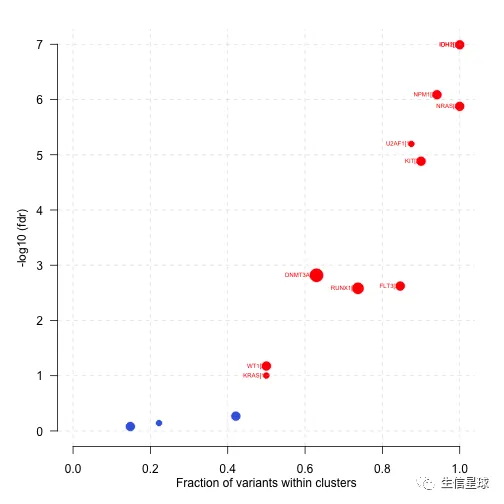
图中点的大小对应基因内突变cluster的数量,x轴是这些cluster中突变数量或比例。上图中,IDH1的18个mutation都存在于1个cluster中,所以显示的基因名后面的括号中显示1
什么是mutation cluster?(来自https://www.ncbi.nlm.nih.gov/pmc/articles/PMC4710516/) An important biological consequence of non-uniform distribution of mutations is that a disproportionately large number of changes can accumulate in a limited section of a genome, forming a mutation cluster
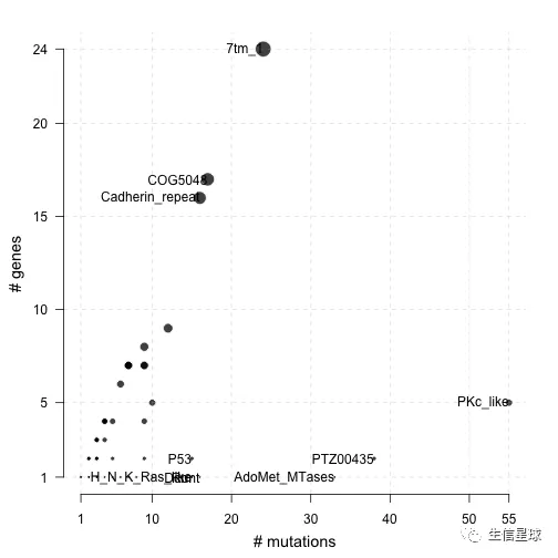
5.3 蛋白结构域注释 | pfamDomains
Pfam 数据库是蛋白结构域注释数据库,它使用基于隐马尔可夫模型的多序列比对方法对蛋白质序列进行家族分类。分为Pfam-A与Pfam-B两个库:
Pfam-A:包含经人工编辑,有完整注释的高质量记录条目
Pfam-B:计算机工具自动编辑,除Pfam-A外的条目,质量较低
这里,可以利用pfamDomains来看看氨基酸改变区域的结构域信息,帮助了解给定的癌症队列中,哪些结构域是经常被影响的。
下图中,圆点表示结构域,x轴是该结构域内存在的突变数量,y轴和圆点的大小是影响的基因数量
# 选择突变最多的10个pfam domain
laml.pfam = pfamDomains(maf = laml, AACol = 'Protein_Change', top = 10)
#Protein summary (Printing first 7 columns for display convenience)
laml.pfam$proteinSummary[,1:7, with = FALSE]
##         HGNC AAPos Variant_Classification  N total
##    1: DNMT3A   882      Missense_Mutation 27    54
##    2:   IDH1   132      Missense_Mutation 18    18
##    3:   IDH2   140      Missense_Mutation 17    20
##    4:   FLT3   835      Missense_Mutation 14    52
##    5:   FLT3   599           In_Frame_Ins 10    52
##   ---
## 1512: ZNF646   875      Missense_Mutation  1     1
## 1513: ZNF687   554      Missense_Mutation  1     2
## 1514: ZNF687   363      Missense_Mutation  1     2
## 1515: ZNF75D     5      Missense_Mutation  1     1
## 1516: ZNF827   427        Frame_Shift_Del  1     1
##        fraction   DomainLabel
##    1: 0.5000000 AdoMet_MTases
##    2: 1.0000000      PTZ00435
##    3: 0.8500000      PTZ00435
##    4: 0.2692308      PKc_like
##    5: 0.1923077      PKc_like
##   ---
## 1512: 1.0000000          <NA>
## 1513: 0.5000000          <NA>
## 1514: 0.5000000          <NA>
## 1515: 1.0000000          <NA>
## 1516: 1.0000000          <NA>
#Domain summary (Printing first 3 columns for display convenience)
laml.pfam$domainSummary[,1:3, with = FALSE]
##        DomainLabel nMuts nGenes
##   1:      PKc_like    55      5
##   2:      PTZ00435    38      2
##   3: AdoMet_MTases    33      1
##   4:         7tm_1    24     24
##   5:       COG5048    17     17
##  ---
## 499:    ribokinase     1      1
## 500:   rim_protein     1      1
## 501: sigpep_I_bact     1      1
## 502:           trp     1      1
## 503:        zf-BED     1      1
5.4 生存分析 | Survival analysis
mafSurvival函数可以根据我们自己定义的基因突变情况进行分组,或者自定义样本进行分组,来绘制KM plot。需要输入数据包含 Tumor_Sample_Barcode (要和MAF文件的对应), binary event (1/0), time to event
利用给定基因进行分组,看看突变与不突变的生存差异
#Survival analysis based on grouping of DNMT3A mutation status
# 参数time表示随访时间
# 参数Status表示生存状态
mafSurvival(maf = laml, genes = 'DNMT3A', time = 'days_to_last_followup', Status = 'Overall_Survival_Status', isTCGA = TRUE)
## DNMT3A
##     48
##     Group medianTime   N
## 1: Mutant        245  45
## 2:     WT        396 137
参数isTCGA在这里设定数据是否来自TCGA,看源代码会发现这么一句,表示如果是来自TCGA的数据,临床信息会将前12个字符提取出来,用于和MAF对应:
if (isTCGA) {
        clinicalData$Tumor_Sample_Barcode = substr(x = clinicalData$Tumor_Sample_Barcode,
            start = 1, stop = 12)
    }
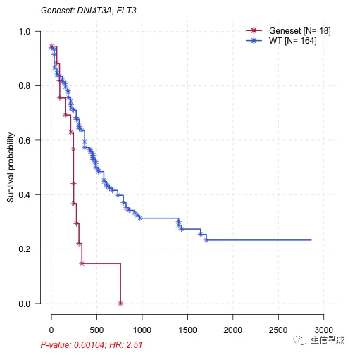
与预后较差有关基因集的预测
#Using top 20 mutated genes to identify a set of genes (of size 2) to predict poor prognostic groups
prog_geneset = survGroup(maf = laml, top = 20, geneSetSize = 2, time = "days_to_last_followup", Status = "Overall_Survival_Status", verbose = FALSE)
print(prog_geneset)
##     Gene_combination P_value    hr  WT Mutant
##  1:      FLT3_DNMT3A 0.00104 2.510 164     18
##  2:      DNMT3A_SMC3 0.04880 2.220 176      6
##  3:      DNMT3A_NPM1 0.07190 1.720 166     16
##  4:      DNMT3A_TET2 0.19600 1.780 176      6
##  5:        FLT3_TET2 0.20700 1.860 177      5
##  6:        NPM1_IDH1 0.21900 0.495 176      6
##  7:      DNMT3A_IDH1 0.29300 1.500 173      9
##  8:       IDH2_RUNX1 0.31800 1.580 176      6
##  9:        FLT3_NPM1 0.53600 1.210 165     17
## 10:      DNMT3A_IDH2 0.68000 0.747 178      4
## 11:      DNMT3A_NRAS 0.99200 0.986 178      4
其中p<0.05表示预后较差,可以选其中一个基因集来看看
mafSurvGroup(maf = laml, geneSet = c("DNMT3A", "FLT3"), time = "days_to_last_followup", Status = "Overall_Survival_Status")
##     Group medianTime   N
## 1: Mutant      242.5  18
## 2:     WT      379.5 164
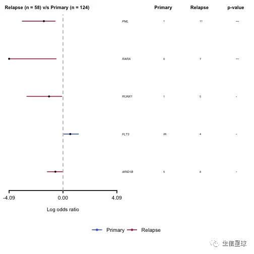
5.5 比较两个MAF文件 | mafComapre
不同癌症、同种癌症的不同时期之间,或者不同性别之间,它们的突变模式(mutation pattern)是不同的,我们可以比较两个不同的队列(maf文件)来检测这些差异的突变基因。反正只要能明确分组,就可以进行比较
例如:急性早幼粒细胞白血病(Acute Promyelocytic Leukemia)在复发期体现出PML、RARA基因的突变,但是早期没有
这里可以利用mafComapre 对两个不同时期进行fisher检验
#Primary APL MAF
primary.apl = system.file("extdata", "APL_primary.maf.gz", package = "maftools")
primary.apl = read.maf(maf = primary.apl)
## -Reading
## -Validating
## --Non MAF specific values in Variant_Classification column:
##   ITD
## -Silent variants: 45
## -Summarizing
## -Processing clinical data
## --Missing clinical data
## -Finished in 0.088s elapsed (0.080s cpu)
#Relapse APL MAF
relapse.apl = system.file("extdata", "APL_relapse.maf.gz", package = "maftools")
relapse.apl = read.maf(maf = relapse.apl)
## -Reading
## -Validating
## --Non MAF specific values in Variant_Classification column:
##   ITD
## -Silent variants: 19
## -Summarizing
## -Processing clinical data
## --Missing clinical data
## -Finished in 0.102s elapsed (0.076s cpu)
#Considering only genes which are mutated in at-least in 5 samples in one of the cohort to avoid bias due to genes mutated in single sample.
pt.vs.rt <- mafCompare(m1 = primary.apl, m2 = relapse.apl, m1Name = 'Primary', m2Name = 'Relapse', minMut = 5)
print(pt.vs.rt)
## $results
##    Hugo_Symbol Primary Relapse         pval         or
## 1:         PML       1      11 1.529935e-05 0.03537381
## 2:        RARA       0       7 2.574810e-04 0.00000000
## 3:       RUNX1       1       5 1.310500e-02 0.08740567
## 4:        FLT3      26       4 1.812779e-02 3.56086275
## 5:      ARID1B       5       8 2.758396e-02 0.26480490
## 6:         WT1      20      14 2.229087e-01 0.60619329
## 7:        KRAS       6       1 4.334067e-01 2.88486293
## 8:        NRAS      15       4 4.353567e-01 1.85209500
## 9:      ARID1A       7       4 7.457274e-01 0.80869223
##          ci.up      ci.low      adjPval
## 1:   0.2552937 0.000806034 0.0001376942
## 2:   0.3006159 0.000000000 0.0011586643
## 3:   0.8076265 0.001813280 0.0393149868
## 4:  14.7701728 1.149009169 0.0407875250
## 5:   0.9698686 0.064804160 0.0496511201
## 6:   1.4223101 0.263440988 0.3343630535
## 7: 135.5393108 0.337679367 0.4897762916
## 8:   8.0373994 0.553883512 0.4897762916
## 9:   3.9297309 0.195710173 0.7457273717
##
## $SampleSummary
##     Cohort SampleSize
## 1: Primary        124
## 2: Relapse         58
从表中可以看到PML和RARA都是在复发期的突变更多,可以作图再看看:
# 森林图
forestPlot(mafCompareRes = pt.vs.rt, pVal = 0.1, color = c('royalblue', 'maroon'), geneFontSize = 0.5)
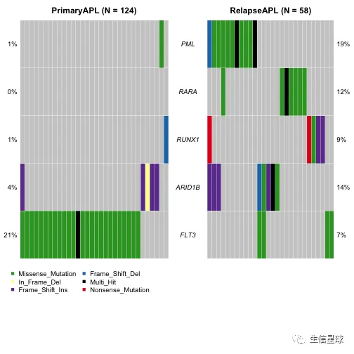
# 还可以把这些基因在不同时期的突变画一个瀑布图
genes = c("PML", "RARA", "RUNX1", "ARID1B", "FLT3")
coOncoplot(m1 = primary.apl, m2 = relapse.apl, m1Name = 'PrimaryAPL', m2Name = 'RelapseAPL', genes = genes, removeNonMutated = TRUE)
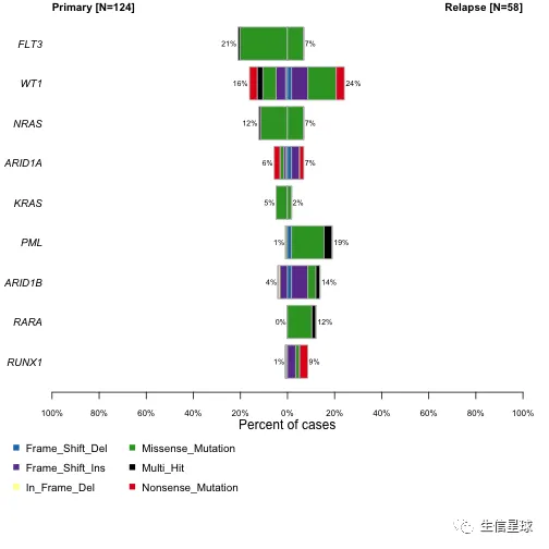
# 或者条形图
coBarplot(m1 = primary.apl, m2 = relapse.apl, m1Name = "Primary", m2Name = "Relapse")
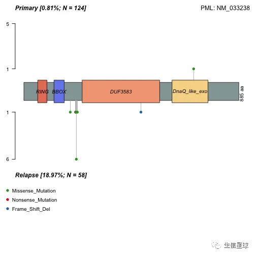
# 还能看看不同分组之间的突变位点和类型
lollipopPlot2(m1 = primary.apl, m2 = relapse.apl, gene = "PML", AACol1 = "amino_acid_change", AACol2 = "amino_acid_change", m1_name = "Primary", m2_name = "Relapse")
##    HGNC refseq.ID protein.ID aa.length
## 1:  PML NM_033238  NP_150241       882
## 2:  PML NM_002675  NP_002666       633
## 3:  PML NM_033249  NP_150252       585
## 4:  PML NM_033247  NP_150250       435
## 5:  PML NM_033239  NP_150242       829
## 6:  PML NM_033250  NP_150253       781
## 7:  PML NM_033240  NP_150243       611
## 8:  PML NM_033244  NP_150247       560
## 9:  PML NM_033246  NP_150249       423
5.6 临床富集分析 | clinicalEnrichment
拿到临床信息中的某个特征,然后看看出现了哪些突变
这个函数clinicalEnrichment()采用Fisher精确检验,会进行两两比较(比如M1和M2,M1和M3),以及分组比较(比如M1和其他各组集合),结果分别存放在pairwise_comparision和groupwise_comparision
fab.ce = clinicalEnrichment(maf = laml, clinicalFeature = 'FAB_classification')
##
## M0 M1 M2 M3 M4 M5 M6 M7
## 19 44 44 21 39 19  3  3
# 两两比较结果
head(fab.ce$pairwise_comparision)
##    Hugo_Symbol Feature_1 Feature_2 n_mutated_Feature1
## 1:        TP53        M7        M1             3 of 3
## 2:        TP53        M7        M3             3 of 3
## 3:        TP53        M7        M5             3 of 3
## 4:        TP53        M7        M4             3 of 3
## 5:        TP53        M7        M2             3 of 3
## 6:      DNMT3A        M5        M3           10 of 19
##    n_mutated_Feature2         fdr
## 1:            2 of 44 0.005844156
## 2:            0 of 21 0.005844156
## 3:            0 of 19 0.005844156
## 4:            2 of 39 0.005879791
## 5:            3 of 44 0.006660500
## 6:            1 of 21 0.028683522
#分组比较结果 Significant associations p-value < 0.05
fab.ce$groupwise_comparision[p_value < 0.05]
##    Hugo_Symbol Group1 Group2 n_mutated_group1
## 1:        IDH1     M1   Rest         11 of 44
## 2:        TP53     M7   Rest           3 of 3
## 3:      DNMT3A     M5   Rest         10 of 19
## 4:       CEBPA     M2   Rest          7 of 44
## 5:       RUNX1     M0   Rest          5 of 19
## 6:        NPM1     M5   Rest          7 of 19
## 7:        NPM1     M3   Rest          0 of 21
## 8:      DNMT3A     M3   Rest          1 of 21
##    n_mutated_group2      p_value       OR      OR_low
## 1:         7 of 149 0.0002597371 6.670592 2.173829026
## 2:        12 of 190 0.0003857187      Inf 5.355415451
## 3:        38 of 174 0.0089427384 3.941207 1.333635173
## 4:         6 of 149 0.0117352110 4.463237 1.204699322
## 5:        11 of 174 0.0117436825 5.216902 1.243812880
## 6:        26 of 174 0.0248582372 3.293201 1.001404899
## 7:        33 of 172 0.0278630823 0.000000 0.000000000
## 8:        47 of 172 0.0294005111 0.133827 0.003146708
##       OR_high       fdr
## 1: 21.9607250 0.0308575
## 2:        Inf 0.0308575
## 3: 11.8455979 0.3757978
## 4: 17.1341278 0.3757978
## 5: 19.4051505 0.3757978
## 6: 10.1210509 0.5880102
## 7:  0.8651972 0.5880102
## 8:  0.8848897 0.5880102
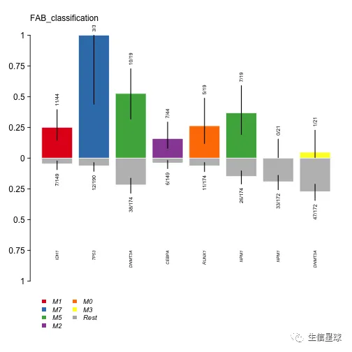
看到IDH1 突变主要发生在M1亚型中 ,同理DNMT3A在M5,TP53在M7。这些信息也能进行可视化
plotEnrichmentResults(enrich_res = fab.ce, pVal = 0.05, geneFontSize = 0.5, annoFontSize = 0.6)
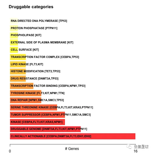
5.7 药物基因互作 | drugInteractions
它可以查询DGIdb数据库(Drug-Gene Interaction database),用来分析药物-基因作用以及基因的成药性(gene druggability)。不过这里只是用于研究,不能用于临床
DGIdb是一个药物-基因相互作用数据库,其中主要是癌基因,当然也不乏其他健康相关的基因(如心脏病、糖尿病、阿尔兹海默症)。DGIdb contains over 40,000 genes and 10,000 drugs involved in over 100,000 drug-gene interactions or belonging to one of 42 potentially druggable gene categories.
# 显示潜在可成药基因(少于5个基因就全部显示,多于5个就显示前5个)
dgi = drugInteractions(maf = laml, fontSize = 0.75)
# 提供基因名,返回互作的药物
dnmt3a.dgi = drugInteractions(genes = "DNMT3A", drugs = TRUE)
## Number of claimed drugs for given genes:
##      Gene N
## 1: DNMT3A 7
#Printing selected columns.
dnmt3a.dgi[,.(Gene, interaction_types, drug_name, drug_claim_name)]
##      Gene interaction_types    drug_name drug_claim_name
## 1: DNMT3A                                            N/A
## 2: DNMT3A                   DAUNORUBICIN    Daunorubicin
## 3: DNMT3A                     DECITABINE      Decitabine
## 4: DNMT3A                     IDARUBICIN      IDARUBICIN
## 5: DNMT3A                     DECITABINE      DECITABINE
## 6: DNMT3A         inhibitor   DECITABINE   CHEMBL1201129
## 7: DNMT3A         inhibitor  AZACITIDINE      CHEMBL1489
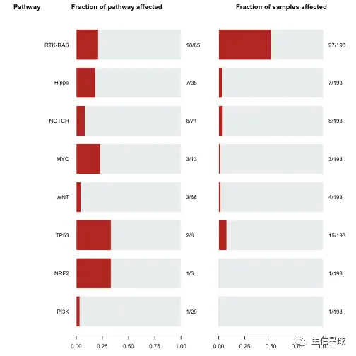
5.8 致癌信号通路 | OncogenicPathways
OncogenicPathways(maf = laml)
##    Pathway  N n_affected_genes fraction_affected
## 1:    PI3K 29                1        0.03448276
## 2:    NRF2  3                1        0.33333333
## 3:    TP53  6                2        0.33333333
## 4:     WNT 68                3        0.04411765
## 5:     MYC 13                3        0.23076923
## 6:   NOTCH 71                6        0.08450704
## 7:   Hippo 38                7        0.18421053
## 8: RTK-RAS 85               18        0.21176471
##    Mutated_samples Fraction_mutated_samples
## 1:               1              0.005181347
## 2:               1              0.005181347
## 3:              15              0.077720207
## 4:               4              0.020725389
## 5:               3              0.015544041
## 6:               8              0.041450777
## 7:               7              0.036269430
## 8:              97              0.502590674
# 例如:RTK-RAS这个pathway中所有基因突变情况
PlotOncogenicPathways(maf = laml, pathways = "RTK-RAS")

其中抑癌基因是红色,致癌基因是蓝色
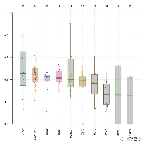
5.9 肿瘤异质性和MATH分数 | inferHeterogeneity
肿瘤是普遍存在异质性的,例如包含多个克隆。这种异质性可以通过等位基因频率( variant allele frequencies, VAF)的聚类进行推断。
关于等位基因频率(VAF)(来自:t.ly/nDvy): 如果在某种群中一个等位基因的基因频率为20%,那么在种群的所有成员中,1/5的染色体带有那个等位基因,而其他4/5的染色体带有该等位基因的其他对应变种——可以是一种也可以是很多种 (来自:https://doi.org/10.1186/s13073-019-0664-4) The variant allele frequency (VAF; also known as variant allele fraction) is used to infer whether a variant comes from somatic cells or inherited from parents when a matched normal sample is not provided. A variant is potentially a germline mutation if the VAF is approximately 50% or 100%.
这个聚类操作会使用mclust,函数会寻找带有VAF信息的一列(当然可以用vafCol来指定)
library("mclust")
tcga.ab.2972.het = inferHeterogeneity(maf = laml, tsb = 'TCGA-AB-2972', vafCol = 'i_TumorVAF_WU')
# 各突变基因的VAF数据
print(tcga.ab.2972.het$clusterData)
##     Hugo_Symbol Chromosome Start_Position End_Position
##  1:       HMCN1          1      185958621    185958621
##  2:       TUFT1          1      151546791    151546791
##  3:       DNAH5          5       13894834     13894834
##  4:       DOCK2          5      169127134    169127134
##  5:      RNASEN          5       31409392     31409392
##  6:    KIAA0240          6       42797687     42797687
##  7:   C10orf118         10      115891901    115891901
##  8:       FANCI         15       89847119     89847119
##  9:       DNAH3         16       20994057     20994057
## 10:      ZC3H18         16       88688690     88688690
## 11:       ZNF43         19       21991712     21991712
## 12:       MORC3         21       37711165     37711165
## 13:      ATP1B4         23      119505057    119505057
## 14:       STAG2         23      123197716    123197716
## 15:       RIMS1          6       72806854     72806854
## 16:      LARP4B         10         871204       871204
## 17:      PTPN11         12      112926884    112926884
## 18:       SFRS6         20       42088521     42088521
## 19:        ASTL          2       96801149     96801149
##     Tumor_Sample_Barcode  t_vaf cluster     MATH
##  1:         TCGA-AB-2972 0.4858       2 11.62157
##  2:         TCGA-AB-2972 0.4328       2 11.62157
##  3:         TCGA-AB-2972 0.4473       2 11.62157
##  4:         TCGA-AB-2972 0.4021       2 11.62157
##  5:         TCGA-AB-2972 0.4422       2 11.62157
##  6:         TCGA-AB-2972 0.4363       2 11.62157
##  7:         TCGA-AB-2972 0.4843       2 11.62157
##  8:         TCGA-AB-2972 0.4395       2 11.62157
##  9:         TCGA-AB-2972 0.4715       2 11.62157
## 10:         TCGA-AB-2972 0.4315       2 11.62157
## 11:         TCGA-AB-2972 0.4891       2 11.62157
## 12:         TCGA-AB-2972 0.4425       2 11.62157
## 13:         TCGA-AB-2972 0.4300       2 11.62157
## 14:         TCGA-AB-2972 0.4603       2 11.62157
## 15:         TCGA-AB-2972 0.1985       1 11.62157
## 16:         TCGA-AB-2972 0.2704       1 11.62157
## 17:         TCGA-AB-2972 0.2516       1 11.62157
## 18:         TCGA-AB-2972 0.2614       1 11.62157
## 19:         TCGA-AB-2972 0.3695 outlier 11.62157
##     MedianAbsoluteDeviation
##  1:                    3.42
##  2:                    3.42
##  3:                    3.42
##  4:                    3.42
##  5:                    3.42
##  6:                    3.42
##  7:                    3.42
##  8:                    3.42
##  9:                    3.42
## 10:                    3.42
## 11:                    3.42
## 12:                    3.42
## 13:                    3.42
## 14:                    3.42
## 15:                    3.42
## 16:                    3.42
## 17:                    3.42
## 18:                    3.42
## 19:                    3.42
# 聚类结果
print(tcga.ab.2972.het$clusterMeans)
##    Tumor_Sample_Barcode cluster   meanVaf
## 1:         TCGA-AB-2972       2 0.4496571
## 2:         TCGA-AB-2972       1 0.2454750
## 3:         TCGA-AB-2972 outlier 0.3695000
# 可视化
plotClusters(clusters = tcga.ab.2972.het)
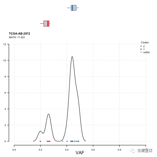
上图很明显分成2群,说明可能存在2个克隆。一群的mean variant allele frequencies为45%左右(为主克隆),另一群是25%左右。
虽然这里可能通过数据分布来直观判断,但是没办法具体量化。因此还可以看:Mutant-Allele Tumor Heterogeneity (MATH)
MATH is a simple quantitative measure of intra-tumor heterogeneity, which calculates the width of the vaf distribution.(即量化VAF分布的离散程度) MATH值越高,预后越差 (计算方法来自:https://www.ncbi.nlm.nih.gov/pmc/articles/PMC5441963/) The MATH score is calculated as 100 × median absolute deviation (MAD)/median of the variant allele frequencies, and describes the ratio of the width of the data to the center of the distribution
考虑一个特殊情况:拷贝数变异
突变基因的拷贝数变异一般范围会影响到VAF的计算,可能会出现异常高/低,从而影响
拷贝数变异(Copy number variation, CNV),是由基因组发生重排而导致的,一般指长度1Kb-3Mb 的基因组大片段的拷贝数增加或者减少(多数 CNV 低于 500kb),是基因组结构变异(Structural variation, SV) 的重要组成部分。CNV变异是人类最常见的变异形式。
CNV数据可以通过 DNACopy的Circular Binary Segmentation方法得到Copy Number Segment文件
suppressMessages(library(dplyr))
seg = system.file('extdata', 'TCGA.AB.3009.hg19.seg.txt', package = 'maftools')
read.table(seg) %>% head()
##             V1         V2      V3       V4         V5
## 1       Sample Chromosome   Start      End Num_Probes
## 2 TCGA-AB-3009          1   61735    86341         15
## 3 TCGA-AB-3009          1   98588  3166089        717
## 4 TCGA-AB-3009          1 3169157  9308037       3956
## 5 TCGA-AB-3009          1 9315847  9404980         60
## 6 TCGA-AB-3009          1 9406979 12845863       1777
##             V6
## 1 Segment_Mean
## 2       -0.683
## 3       0.3069
## 4       0.0039
## 5       0.2934
## 6       0.0104
tcga.ab.3009.het = inferHeterogeneity(maf = laml, tsb = 'TCGA-AB-3009', segFile = seg, vafCol = 'i_TumorVAF_WU')
##    Hugo_Symbol Chromosome Start_Position End_Position
## 1:        PHF6         23      133551224    133551224
##    Tumor_Sample_Barcode     t_vaf Segment_Start
## 1:         TCGA-AB-3009 0.9349112            NA
##    Segment_End Segment_Mean CN
## 1:          NA           NA NA
##    Hugo_Symbol Chromosome Start_Position End_Position
## 1:     NFKBIL2          8      145668658    145668658
## 2:         NF1         17       29562981     29562981
## 3:       SUZ12         17       30293198     30293198
##    Tumor_Sample_Barcode     t_vaf Segment_Start
## 1:         TCGA-AB-3009 0.4415584     145232496
## 2:         TCGA-AB-3009 0.8419000      29054355
## 3:         TCGA-AB-3009 0.8958333      29054355
##    Segment_End Segment_Mean       CN    cluster
## 1:   145760746       0.3976 2.634629 CN_altered
## 2:    30363868      -0.9157 1.060173 CN_altered
## 3:    30363868      -0.9157 1.060173 CN_altered
# 根据这个segment文件,函数就会将没有CNV的基因作为离群值,并且标记出有CNV突变的基因
plotClusters(clusters = tcga.ab.3009.het, genes = 'CN_altered', showCNvars = TRUE)
上图中,NF1和SUZ12基因就存在较高的VAF,这是因为出现了CNV(deletion)。为什么说是出现了deletion,是因为上面的结果中:segment mean这一列
来自: https://docs.gdc.cancer.gov/Data/Bioinformatics_Pipelines/CNV_Pipeline/ The copy number variation (CNV) pipeline uses Affymetrix SNP 6.0 array data to identify genomic regions that are repeated and infer the copy number of these repeats. Diploid regions will have a segment mean of zero, amplified regions will have positive values, and deletions will have negative values.
5.10 突变特征/频谱 | Mutational Signatures
首先,什么是突变特征/频谱?
每种癌症在发展过程中,都会出现一些比较特有的碱基替换,可以认为是一种特征(signature),并且这种特征只是针对于somatic 的mutation,一般一个样本也就几百个somatic 的mutation。somatic突变在全基因组上发生的比例约百万分之一,如果是全基因组肿瘤基因测序, 可能会有3万个左右的somatic突变,如果是全外显子测序,是300个左右。
在http://www.nature.com/nature/journal/v500/n7463/full/nature12477.html这篇文章中,研究了4,938,362 mutations from 7,042 cancers样本;研究了30种癌症,发现21种不同的mutation signature
COSMIC的30个突变特征
来自(https://cancer.sanger.ac.uk/cosmic/signatures): Somatic mutations are present in all cells of the human body and occur throughout life. Different mutational processes generate unique combinations of mutation types, termed “Mutational Signatures”.
sanger研究所科学家提出来了肿瘤somatic突变的signature概念 ,把96突变频谱的非负矩阵分解后的30个特征。R包deconstructSigs可以把自己的96突变频谱对应到cosmic数据库的30个突变特征,不同的特征有不同的生物学含义
它的30个signature的96突变频谱在:https://cancer.sanger.ac.uk/cancergenome/assets/signatures_probabilities.txt
cosmic=read.table('https://cancer.sanger.ac.uk/cancergenome/assets/signatures_probabilities.txt',
                  header = T,sep = '\t')[,1:33]
head(cosmic[,1:3])
tmp=cosmic[,2];substr(tmp,2,2) <- '.'
rownames(cosmic)=paste(gsub('>','',cosmic[,1]),
      tmp)
96突变频谱是怎么回事?
看这个图:https://en.wikipedia.org/wiki/Mutational_signatures
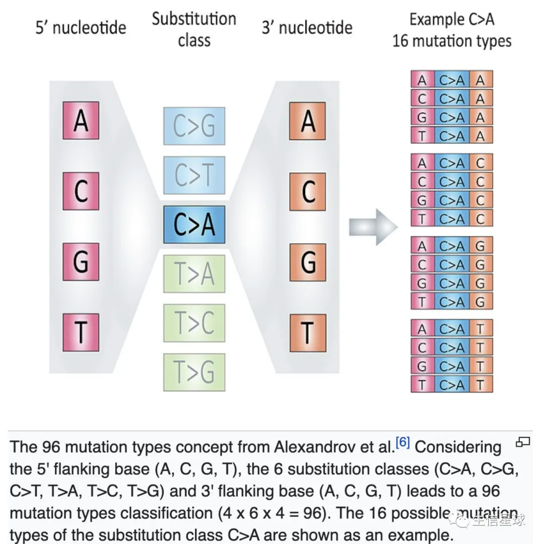
正链上的C->A突变,对应负链上为G->T,因此某个位点的突变可以划分为6种:
C>A, 表示C>A和G>T两种 C>G, 表示C>G和G>C两种 C>T, 表示C>T和G>A两种 T>A,表示T>A和A>T两种 T>C,表示T>C和A>G两种 T>G,表示T>G和A>C两种
然后在突变位点的上下游各取一个碱基,组成3碱基,所以有4x6x4=96种模式,每种模式的频率分布就是突变频谱。它可以作为一个肿瘤样本的特征,从而进行样本间的比较。比如MutationalPatterns这个R包就可以做这样的分析
我们接下来使用maftools进行计算
#Requires BSgenome object
library(BSgenome.Hsapiens.UCSC.hg19, quietly = TRUE)
laml.tnm = trinucleotideMatrix(maf = laml, prefix = 'chr', add = TRUE, ref_genome = "BSgenome.Hsapiens.UCSC.hg19")
## -Extracting 5' and 3' adjacent bases
## -Extracting +/- 20bp around mutated bases for background C>T estimation
## -Estimating APOBEC enrichment scores
## --Performing one-way Fisher's test for APOBEC enrichment
## ---APOBEC related mutations are enriched in  3.315 % of samples (APOBEC enrichment score > 2 ;  6  of  181  samples)
## -Creating mutation matrix
## --matrix of dimension 188x96
这个计算过程主要分成两部分:
Estimates APOBEC enrichment scores
Prepares a mutational matrix for signature analysis.
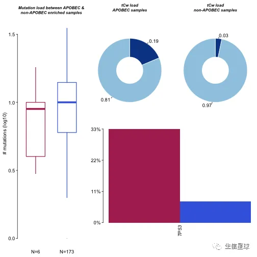
APOBEC富集与非富集样本的差异分析
plotApobecDiff函数可以拿trinucleotideMatrix的APOBED富集分数,然后将样本分成两类:APOBEC enriched and non-APOBEC enriched。之后,鉴定两类之间差异基因
# 这里仅仅是代码示例,LAML并没有APOBEC enrichment,所以不适合做这个分析
plotApobecDiff(tnm = laml.tnm, maf = laml, pVal = 0.2)
## $results
##      Hugo_Symbol Enriched nonEnriched       pval
##   1:        TP53        2          13 0.08175632
##   2:        TET2        1          16 0.45739351
##   3:        FLT3        2          45 0.65523131
##   4:      DNMT3A        1          47 1.00000000
##   5:      ADAM11        0           2 1.00000000
##  ---
## 132:         WAC        0           2 1.00000000
## 133:         WT1        0          12 1.00000000
## 134:      ZBTB33        0           2 1.00000000
## 135:      ZC3H18        0           2 1.00000000
## 136:      ZNF687        0           2 1.00000000
##             or      ci.up     ci.low adjPval
##   1: 5.9976455  46.608861 0.49875432       1
##   2: 1.9407002  18.983979 0.03882963       1
##   3: 1.4081851  10.211621 0.12341748       1
##   4: 0.5335362   4.949499 0.01101929       1
##   5: 0.0000000 164.191472 0.00000000       1
##  ---
## 132: 0.0000000 164.191472 0.00000000       1
## 133: 0.0000000  12.690862 0.00000000       1
## 134: 0.0000000 164.191472 0.00000000       1
## 135: 0.0000000 164.191472 0.00000000       1
## 136: 0.0000000 164.191472 0.00000000       1
##
## $SampleSummary
##         Cohort SampleSize  Mean Median
## 1:    Enriched          6 7.167    6.5
## 2: nonEnriched        172 9.715    9.0
6 小技巧
6.1 MAF取子集
## 常规筛选
#Extract data for samples 'TCGA.AB.3009' and 'TCGA.AB.2933'  (Printing just 5 rows for display convenience)
subsetMaf(maf = laml, tsb = c('TCGA-AB-3009', 'TCGA-AB-2933'), mafObj = FALSE)[1:5]
##    Hugo_Symbol Entrez_Gene_Id           Center
## 1:      ABCB11           8647 genome.wustl.edu
## 2:       ACSS3          79611 genome.wustl.edu
## 3:        ANK3            288 genome.wustl.edu
## 4:       AP1G2           8906 genome.wustl.edu
## 5:         ARC          23237 genome.wustl.edu
##    NCBI_Build Chromosome Start_Position End_Position
## 1:         37          2      169780250    169780250
## 2:         37         12       81536902     81536902
## 3:         37         10       61926581     61926581
## 4:         37         14       24033309     24033309
## 5:         37          8      143694874    143694874
##    Strand Variant_Classification Variant_Type
## 1:      +      Missense_Mutation          SNP
## 2:      +      Missense_Mutation          SNP
## 3:      +            Splice_Site          SNP
## 4:      +      Missense_Mutation          SNP
## 5:      +      Missense_Mutation          SNP
##    Reference_Allele Tumor_Seq_Allele1 Tumor_Seq_Allele2
## 1:                G                 G                 A
## 2:                C                 C                 T
## 3:                C                 C                 A
## 4:                C                 C                 T
## 5:                C                 C                 G
##    Tumor_Sample_Barcode Protein_Change i_TumorVAF_WU
## 1:         TCGA-AB-3009       p.A1283V      46.97218
## 2:         TCGA-AB-3009        p.A266V      47.32510
## 3:         TCGA-AB-3009                     43.99478
## 4:         TCGA-AB-3009        p.R346Q      47.08000
## 5:         TCGA-AB-3009        p.W253C      42.96435
##    i_transcript_name
## 1:       NM_003742.2
## 2:       NM_024560.2
## 3:       NM_020987.2
## 4:       NM_003917.2
## 5:       NM_015193.3
##Same as above but return output as an MAF object (Default behaviour)
subsetMaf(maf = laml, tsb = c('TCGA-AB-3009', 'TCGA-AB-2933'))
## An object of class  MAF
##                    ID          summary Mean Median
##  1:        NCBI_Build               37   NA     NA
##  2:            Center genome.wustl.edu   NA     NA
##  3:           Samples                2   NA     NA
##  4:            nGenes               34   NA     NA
##  5:   Frame_Shift_Ins                5  2.5    2.5
##  6:      In_Frame_Ins                1  0.5    0.5
##  7: Missense_Mutation               26 13.0   13.0
##  8: Nonsense_Mutation                2  1.0    1.0
##  9:       Splice_Site                1  0.5    0.5
## 10:             total               35 17.5   17.5
## 指定query筛选
#Select all Splice_Site mutations from DNMT3A and NPM1
subsetMaf(maf = laml, genes = c('DNMT3A', 'NPM1'), mafObj = FALSE,query = "Variant_Classification == 'Splice_Site'")
##    Hugo_Symbol Entrez_Gene_Id           Center
## 1:      DNMT3A           1788 genome.wustl.edu
## 2:      DNMT3A           1788 genome.wustl.edu
## 3:      DNMT3A           1788 genome.wustl.edu
## 4:      DNMT3A           1788 genome.wustl.edu
## 5:      DNMT3A           1788 genome.wustl.edu
## 6:      DNMT3A           1788 genome.wustl.edu
##    NCBI_Build Chromosome Start_Position End_Position
## 1:         37          2       25459874     25459874
## 2:         37          2       25467208     25467208
## 3:         37          2       25467022     25467022
## 4:         37          2       25459803     25459803
## 5:         37          2       25464576     25464576
## 6:         37          2       25469029     25469029
##    Strand Variant_Classification Variant_Type
## 1:      +            Splice_Site          SNP
## 2:      +            Splice_Site          SNP
## 3:      +            Splice_Site          SNP
## 4:      +            Splice_Site          SNP
## 5:      +            Splice_Site          SNP
## 6:      +            Splice_Site          SNP
##    Reference_Allele Tumor_Seq_Allele1 Tumor_Seq_Allele2
## 1:                C                 C                 G
## 2:                C                 C                 T
## 3:                A                 A                 G
## 4:                A                 A                 C
## 5:                C                 C                 A
## 6:                C                 C                 A
##    Tumor_Sample_Barcode Protein_Change i_TumorVAF_WU
## 1:         TCGA-AB-2818        p.R803S         36.84
## 2:         TCGA-AB-2822                        62.96
## 3:         TCGA-AB-2891                        34.78
## 4:         TCGA-AB-2898                        46.43
## 5:         TCGA-AB-2934        p.G646V         37.50
## 6:         TCGA-AB-2968        p.E477*         40.00
##    i_transcript_name
## 1:       NM_022552.3
## 2:       NM_022552.3
## 3:       NM_022552.3
## 4:       NM_022552.3
## 5:       NM_022552.3
## 6:       NM_022552.3
#Same as above but include only 'i_transcript_name' column in the output
subsetMaf(maf = laml, genes = c('DNMT3A', 'NPM1'), mafObj = FALSE, query = "Variant_Classification == 'Splice_Site'", fields = 'i_transcript_name')
##    Hugo_Symbol Chromosome Start_Position End_Position
## 1:      DNMT3A          2       25459874     25459874
## 2:      DNMT3A          2       25467208     25467208
## 3:      DNMT3A          2       25467022     25467022
## 4:      DNMT3A          2       25459803     25459803
## 5:      DNMT3A          2       25464576     25464576
## 6:      DNMT3A          2       25469029     25469029
##    Reference_Allele Tumor_Seq_Allele2
## 1:                C                 G
## 2:                C                 T
## 3:                A                 G
## 4:                A                 C
## 5:                C                 A
## 6:                C                 A
##    Variant_Classification Variant_Type
## 1:            Splice_Site          SNP
## 2:            Splice_Site          SNP
## 3:            Splice_Site          SNP
## 4:            Splice_Site          SNP
## 5:            Splice_Site          SNP
## 6:            Splice_Site          SNP
##    Tumor_Sample_Barcode i_transcript_name
## 1:         TCGA-AB-2818       NM_022552.3
## 2:         TCGA-AB-2822       NM_022552.3
## 3:         TCGA-AB-2891       NM_022552.3
## 4:         TCGA-AB-2898       NM_022552.3
## 5:         TCGA-AB-2934       NM_022552.3
## 6:         TCGA-AB-2968       NM_022552.3
## 按临床信息筛选
#Select all samples with FAB clasification M4 in clinical data
laml_m4 = subsetMaf(maf = laml, clinQuery = "FAB_classification %in% 'M4'")
6.2 拿到已经做好的TCGA MAF
https://github.com/PoisonAlien/TCGAmutations
数据来自(TCGA firehose)[http://firebrowse.org/] and (TCGA MC3)[https://gdc.cancer.gov/about-data/publications/mc3-2017] projects. Every dataset is stored as an MAF object containing somatic mutations along with clinical information.
# 安装(但是我目前安装不上)
# BiocManager::install(pkgs = "PoisonAlien/TCGAmutations")

# 加载 TCGA LUAD cohort. Note that by default MAF from MC3 study is returned
TCGAmutations::tcga_load(study = "LUAD")

# 切换数据源
TCGAmutations::tcga_load(study = "LUAD", source = "Firehose")