090-转录组差异分析金标准-Limma-voom实战
刘小泽写于19.3.11
Limma作为差异分析的“金标准”最初是应用在芯片数据分析中,voom的功能是为了RNA-Seq的分析产生的。详细探索一下limma的功能吧
本次的测试数据可以在公众号回复voom获得
Limma-voom强大在于三个方面:
- False discovery rate比较低(准确性),异常值影响小
- 假阳性控制不错
- 运算很快
配置信息
> library(edgeR)
Loading required package: limma
> counts <- read.delim("all_counts.txt", row.names = 1)
> head(counts[1:3,1:3])
          C61 C62 C63
AT1G01010 341 371 275
AT1G01020 164  94 176
AT1G03987   0   0   0
> dim(counts)
[1] 32833    24
# 构建DGEList对象,将counts和sample信息包含进去
> d0 <- DGEList(counts)
预处理
> # 计算标准化因子
> d0 <- calcNormFactors(d0)
> d0
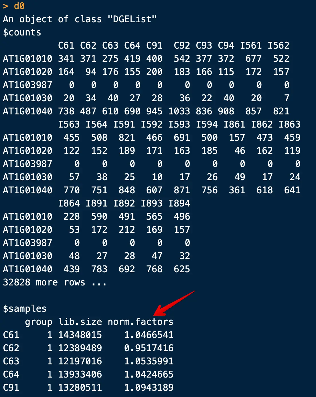
注意,这里的calcNormFactors并不是进行了标准化,仅仅是计算了一个参数,用于下游标准化
# 过滤低表达基因[阈值根据自己需要设定]
cutoff <- 1
cut <- which(apply(cpm(d0), 1, max) < cutoff)
d <- d0[-cut,]
dim(d)
[1] 21081    24
# 剩下 21081个基因
然后根据列名提取样本信息(sample name)
> spname <- colnames(counts)
> spname
 [1] "C61"  "C62"  "C63"  "C64"  "C91"  "C92"  "C93"
 [8] "C94"  "I561" "I562" "I563" "I564" "I591" "I592"
[15] "I593" "I594" "I861" "I862" "I863" "I864" "I891"
[22] "I892" "I893" "I894"
看到样本是按照两个因素(品系C/I5/I8、时间6/9)分类的,并且四个生物学重复写在了最后C/I5/I8 | 6/9 | 1/2/3/4
> # 分离出分组信息
> strain <- substr(spname, 1, nchar(spname) - 2)
> time <- substr(spname, nchar(spname) - 1, nchar(spname) - 1)
> strain
 [1] "C"  "C"  "C"  "C"  "C"  "C"  "C"  "C"  "I5" "I5"
[11] "I5" "I5" "I5" "I5" "I5" "I5" "I8" "I8" "I8" "I8"
[21] "I8" "I8" "I8" "I8"
> time
 [1] "6" "6" "6" "6" "9" "9" "9" "9" "6" "6" "6" "6"
[13] "9" "9" "9" "9" "6" "6" "6" "6" "9" "9" "9" "9"
再将这两部分整合进group分组信息中
> # 再将这两部分整合进group分组信息中[生成因子型向量]
> group <- interaction(strain, time)
> group
 [1] C.6  C.6  C.6  C.6  C.9  C.9  C.9  C.9  I5.6 I5.6
[11] I5.6 I5.6 I5.9 I5.9 I5.9 I5.9 I8.6 I8.6 I8.6 I8.6
[21] I8.9 I8.9 I8.9 I8.9
Levels: C.6 I5.6 I8.6 C.9 I5.9 I8.9
当然,也可以自己手动输入或从其他文件导入,但必须注意一点:这个group metadata必须和counts的列明顺序对应
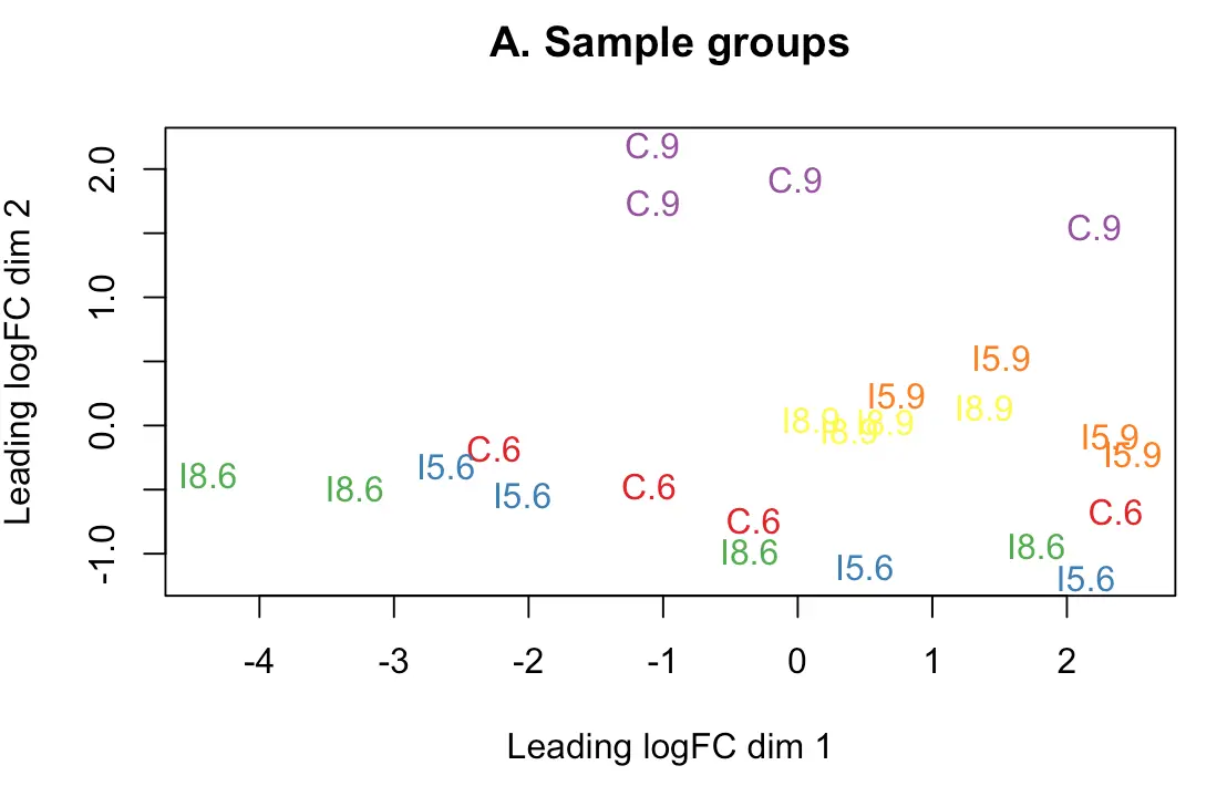
多个实验因子同时存在时,要进行MDS(multidimensional scaling)分析,即“多维尺度变换”。正式差异分析前帮助我们判断潜在的差异样本,结果会将所有样本划分成几个维度,第一维度的样本代表了最大的差异
> # Multidimensional scaling (MDS) plot
> suppressMessages(library(RColorBrewer))
> col.group <- group
> levels(col.group) <- brewer.pal(nlevels(col.group), "Set1")
> col.group <- as.character(col.group)
> plotMDS(d, labels=group, col=col.group)
> title(main="A. Sample groups")
Voom转换及方差权重计算
> mm <- model.matrix(~0 + group)
> y <- voom(d, mm, plot = T)
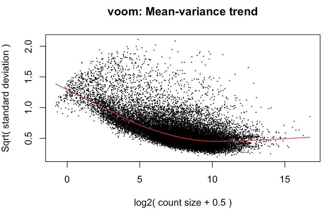
voom到底做了什么转换?
首先原始counts转换成log2的CPM(counts per million reads ),这里的per million reads是根据之前calcNormFactors计算的norm.factors进行规定的;
然后根据每个基因的log2CPM制作了线性模型,并计算了 残差 ;
然后利用了平均表达量(红线)拟合了sqrt(residual standard deviation);
最后得到的平滑曲线可以用来得到每个基因和样本的权重
https://genomebiology.biomedcentral.com/articles/10.1186/gb-2014-15-2-r29
上图效果较好,如果像下面👇这样:就表示数据需要再进行过滤
tmp <- voom(d0, mm, plot = T)
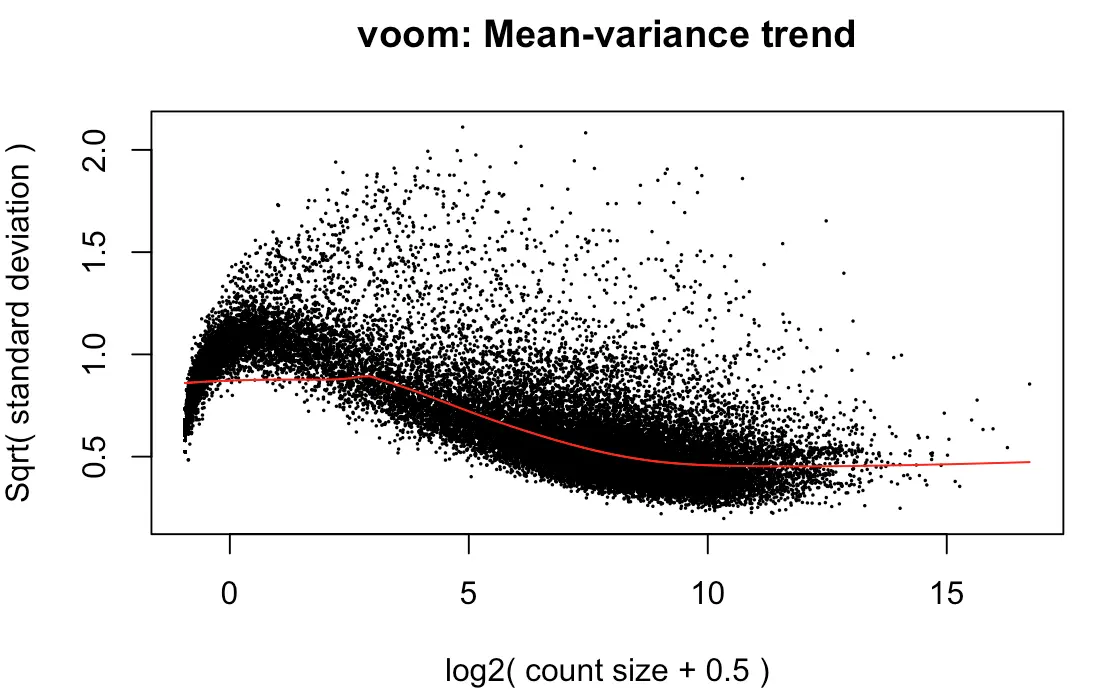
有时我们没有必要弄明白背后复杂的原理,只需要知道如何解释结果:
limma-voom method assumes that rows with zero or very low counts have been removed
如果横坐标接近0的位置出现迅速上升,说明low counts数比较多
Whether your data are “good” or not cannot be determined from this plot
limma的线性拟合模型构建
> fit <- lmFit(y, mm)
> head(coef(fit),3)
          groupC.6 groupI5.6 groupI8.6 groupC.9
AT1G01010 4.685920 5.2477564  4.938939 4.922501
AT1G01020 3.420726 3.4147535  3.130644 3.571855
AT1G01030 1.111114 0.7316936  1.435521 1.157532
          groupI5.9 groupI8.9
AT1G01010  5.382619  5.246093
AT1G01020  3.610579  3.655254
AT1G01030  0.388736  1.222892
组间比较:
例如进行I5品系的6和9小时比较
> contr <- makeContrasts(groupI5.9 - groupI5.6, levels = colnames(coef(fit)))
> contr
           Contrasts
Levels      groupI5.9 - groupI5.6
  groupC.6                      0
  groupI5.6                    -1
  groupI8.6                     0
  groupC.9                      0
  groupI5.9                     1
  groupI8.9                     0
估算组间每个基因的比较:
> tmp <- contrasts.fit(fit, contr)
再利用Empirical Bayes (shrinks standard errors that are much larger or smaller than those from other genes towards the average standard erro)
https://www.degruyter.com/doi/10.2202/1544-6115.1027
> tmp <- eBayes(tmp)
结果中差异基因有哪些呢?
> top.table <- topTable(tmp, sort.by = "P", n = Inf)
> DEG <- na.omit(top.table)
> head(DEG, 5)
              logFC  AveExpr         t      P.Value
AT5G37260  3.163518 6.939588  23.94081 1.437434e-16
AT3G02990  1.646438 3.190750  13.15656 1.610004e-11
AT2G29500 -5.288998 5.471250 -11.94053 9.584101e-11
AT3G24520  1.906690 5.780286  11.80461 1.179985e-10
AT5G65630  1.070550 7.455294  10.86740 5.208111e-10
             adj.P.Val        B
AT5G37260 3.030255e-12 26.41860
AT3G02990 1.697025e-07 15.50989
AT2G29500 6.218818e-07 14.45441
AT3G24520 6.218818e-07 14.52721
AT5G65630 2.195844e-06 13.12701
- logFC: log2 fold change of I5.9/I5.6
- AveExpr: Average expression across all samples, in log2 CPM
- t: logFC divided by its standard error
- P.Value: Raw p-value (based on t) from test that logFC differs from 0
- adj.P.Val: Benjamini-Hochberg false discovery rate adjusted p-value
- B: log-odds that gene is DE (arguably less useful than the other columns)
从前几个差异最显著的基因中可以看到,AT5G37260基因在time9的表达量最高(约time6的8倍),AT2G29500表达量最低,比time6的还少(约1/32)
那么总共有多少差异基因呢?
如果以logFC=2,Pvalue=0.05为阈值进行过滤
> length(which(DEG$adj.P.Val < 0.05 & abs(DEG$logFC)>2 ))
[1] 172
如果要比较其他的组,例如:time6的品系C和品系I5
只需要将makeContrasts修改
contr <- makeContrasts(groupI5.6 - groupC.6, levels = colnames(coef(fit)))
tmp <- contrasts.fit(fit, contr)
tmp <- eBayes(tmp)
top.table <- topTable(tmp, sort.by = "P", n = Inf)
DEG <- na.omit(top.table)
head(DEG, 5)
length(which(DEG$adj.P.Val < 0.05 & abs(DEG$logFC)>2 ))
# 结果只有8个
上面利用了单因子group构建了model matrix,如果存在多个影响因子,可以利用新的因子(就省去了之前因子组合成group的步骤)构建新的矩阵模型
# 构建新的model matrix
> mm <- model.matrix(~strain*time)
> colnames(mm)
[1] "(Intercept)" "strainI5" "strainI8"
[4] "time9" "strainI5:time9" "strainI8:time9"
> y <- voom(d, mm, plot = F)
> fit <- lmFit(y, mm)
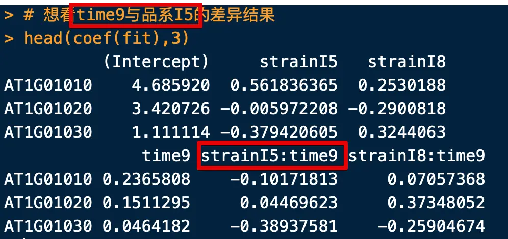
> head(coef(fit),3)
(Intercept) strainI5 strainI8
AT1G01010 4.685920 0.561836365 0.2530188
AT1G01020 3.420726 -0.005972208 -0.2900818
AT1G01030 1.111114 -0.379420605 0.3244063
time9 strainI5:time9 strainI8:time9
AT1G01010 0.2365808 -0.10171813 0.07057368
AT1G01020 0.1511295 0.04469623 0.37348052
AT1G01030 0.0464182 -0.38937581 -0.25904674
- 算法自定义了标准品系为C,标准时间为6(可能是按照字母或数字顺序)
strainI5表示品系I5和标准品系(品系C)在标准时间点(time6)的差异time9表示标准品系(品系C)在time9和time6的差异strainI5:time9表示品系I5和品系C在time9和time6的差异(存在交叉影响)
如果我们想比较品系I5和品系C在time6的差异,就可以:
> tmp <- contrasts.fit(fit, coef = 2)
> tmp <- eBayes(tmp)
> top.table <- topTable(tmp, sort.by = "P", n = Inf)
> DEG <- na.omit(top.table)
> head(DEG, 5)
               logFC    AveExpr          t
AT4G12520 -10.254556  0.3581132 -11.402477
AT3G30720   5.817438  3.3950689  10.528934
AT5G26270   2.421030  4.3788335   9.654257
AT3G33528  -4.780814 -1.8612945  -7.454943
AT1G64795  -4.872595 -1.3119360  -7.079643
               P.Value    adj.P.Val          B
AT4G12520 2.206726e-10 4.651998e-06  3.6958152
AT3G30720 9.108689e-10 9.601014e-06  7.9963406
AT5G26270 4.101051e-09 2.881809e-05 10.8356224
AT3G33528 2.741289e-07 1.444728e-03  0.5677732
AT1G64795 5.985471e-07 2.523594e-03  1.8151705
> length(which(DEG$adj.P.Val < 0.05 & abs(DEG$logFC)>2 ))
[1] 8
可以看到,和之前用单因子group得到的结果一样
但是,这种方法在同时分析交叉影响时就体现出来强大了:
比如我们想看time9与品系I5的差异结果
> # cultivarI5:time9
> tmp <- contrasts.fit(fit, coef = 5)
> tmp <- eBayes(tmp)
> top.table <- topTable(tmp, sort.by = "P", n = Inf)
> DEG <- na.omit(top.table)
> #head(DEG, 5)
> length(which(DEG$adj.P.Val < 0.05 & abs(DEG$logFC)>2 ))
[1] 111
更复杂的模型
有时RNA-Seq需要考虑批次效应(Batch effect)的影响
> batch <- factor(rep(rep(1:2, each = 2), 6))
> batch
 [1] 1 1 2 2 1 1 2 2 1 1 2 2 1 1 2 2 1 1 2 2 1 1 2 2
Levels: 1 2
构建模型时,需要将batch加在最后,其他不变
> mm <- model.matrix(~0 + group + batch)
> y <- voom(d, mm, plot = F)
> fit <- lmFit(y, mm)
> contr <- makeContrasts(groupI5.6 - groupC.6, levels = colnames(coef(fit)))
> tmp <- contrasts.fit(fit, contr)
> tmp <- eBayes(tmp)
> top.table <- topTable(tmp, sort.by = "P", n = Inf)
> DEG <- na.omit(top.table)
> #head(DEG, 5)
> length(which(DEG$adj.P.Val < 0.05 & abs(DEG$logFC)>2 ))
[1] 9
或者需要考虑其他因素的影响,比如这里有一个连续型变量rate,它可能是pH、光照等等对研究材料的影响值
> # Generate example rate data[行数要与count矩阵的列数相等]
> set.seed(10)
> rate <- rnorm(n = 24, mean = 5, sd = 1.7)
> rate
 [1] 5.031868 4.686771 2.668738 3.981415 5.500727
 [6] 5.662650 2.946271 4.381751 2.234656 4.563987
[11] 6.873025 6.284829 4.595003 6.678656 6.260363
[16] 5.151890 3.376595 4.668244 6.573386 5.821063
> # 指定矩阵模型
> mm <- model.matrix(~rate)
> head(mm)
  (Intercept)     rate
1           1 5.031868
2           1 4.686771
3           1 2.668738
4           1 3.981415
5           1 5.500727
6           1 5.662650
> y <- voom(d, mm, plot = F)
> fit <- lmFit(y, mm)
> tmp <- contrasts.fit(fit, coef = 2) # test "rate" coefficient
> tmp <- eBayes(tmp)
> top.table <- topTable(tmp, sort.by = "P", n = Inf)
> DEG <- na.omit(top.table)
> #head(DEG, 5)
> length(which(DEG$adj.P.Val < 0.05 & abs(DEG$logFC)>2 ))
[1] 0
可见rate值并不能成为产生差异基因的原因,但是rate与基因的相关性还是可以探索一下的
> AT1G01060 <- y$E["AT1G01060",]
> plot(AT1G01060 ~ rate, ylim = c(6, 12))
> intercept <- coef(fit)["AT1G01060", "(Intercept)"]
> slope <- coef(fit)["AT1G01060", "rate"]
> abline(a = intercept, b = slope)

图中的斜率就是logFC值,或者可以说每单位rate的增加,gene表达量log2 CPM的改变。这里斜率为-0.096表示:每单位rate的增加,就有-0.096 log2CPM的基因表达量降低;或者每单位rate的增加,就有6.9%的CPM降低(2^0.096 = 1.069)