096-再来看看R中的数据类型
刘小泽写于19.3.29 多掌握一些R的基础知识——数据类型是很有必要的,起码看到别人的代码时不至于懵懵的
什么是Tidy Data?
整天看到花花沉浸Tidyverse不能自拔,我就心想啊,你能给我解释一下什么是Tidy data吗?数据如何才能称作"整洁”?于是花花就说了三句话送我:
- 每个观测占一行
- 每个变量占一列
- 每个值占一个格
就像这样:
##   Students   Subject Years Score
## 1     Mark     Maths     1     5
## 2     Jane   Biology     2     6
## 3 Mohammed   Physics     3     4
## 4      Tom     Maths     2     7
## 5    Celia Computing     3     9
使用tidy数据最大的好处是它的兼容性,比如ggplot完美兼容
既然有tidy,那么什么是untidy呢?
library(tidyverse)
sports<-data.frame(Students=c("Matt", "Matt", "Ellie", "Ellie", "Tim", "Tim", "Louise", "Louise", "Kelly", "Kelly"), Sport=c("Tennis","Tennis", "Rugby", "Rugby","Football", "Football","Swimming","Swimming", "Running", "Running"), Category=c("Wins", "Losses", "Wins", "Losses", "Wins", "Losses", "Wins", "Losses", "Wins", "Losses"), Counts=c(0,1,3,2,1,4,2,2,5,1))
sports

##    Students    Sport Category Counts
## 1      Matt   Tennis     Wins      0
## 2      Matt   Tennis   Losses      1
## 3     Ellie    Rugby     Wins      3
## 4     Ellie    Rugby   Losses      2
## 5       Tim Football     Wins      1
## 6       Tim Football   Losses      4
## 7    Louise Swimming     Wins      2
## 8    Louise Swimming   Losses      2
## 9     Kelly  Running     Wins      5
## 10    Kelly  Running   Losses      1
很明显,一种情况就是:(列中变量过多)untidy的数据在某一列会存在两个变量(比如这里的Wins和Losses)
变量过多就分散seperate一下,需要两个参数:key和value,将包含多个变量的列名赋值给key,将包含多个变量对应值的列名赋值给value就好
spread(sports, key=Category, value=Counts)
##   Students    Sport Losses Wins
## 1    Ellie    Rugby      2    3
## 2    Kelly  Running      1    5
## 3   Louise Swimming      2    2
## 4     Matt   Tennis      1    0
## 5      Tim Football      4    1
另一种情况是:(列中变量过少) 列中没有任何变量,全是值,比如
percentages<-data.frame(student=c("Alejandro", "Pietro", "Jane"), "May"=c(90,12,45), "June"=c(80,30,100))
##    student May June
## 1 Alejandro  90   80
## 2    Pietro  12   30
## 3      Jane  45  100
变量太少就聚集gather一下
gather(percentages, "May", "June", key="Month", value = "Percentage")
##     student Month Percentage
## 1 Alejandro   May         90
## 2    Pietro   May         12
## 3      Jane   May         45
## 4 Alejandro  June         80
## 5    Pietro  June         30
## 6      Jane  June        100
综上,tidy data就是保持"居中”,保证列中的变量有一个就好,发现某一列中变量多了就seperate,变量少了就gather
【R数据科学送给你:http://r4ds.had.co.nz/ 】佩服花花学完了R数据科学整本书
什么是类(Class)?
比如单细胞scater包用的就是Bioconductor的
SingleCellExperiment 就是一个S4类,可以储存/获取spike-in信息、降维数据、每个细胞的size factor、基因/文库元数据等
R数据类型主要有四种:基础型、S3类、S4类、RC型,简单说S3和S4区别是:
我们平常使用 $ 来访问对象就是针对S3类数据(比如数据框、矩阵等),而S4数据中我们使用@
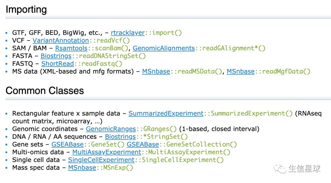
Bioconductor基本就是使用包含数据信息更多的S4类,Bioconductor的官方推荐的类如下:https://www.bioconductor.org/developers/how-to/commonMethodsAndClasses/
S4类创建对象就需要利用自己的一套系统,还是以SingleCellExperiment为例
library(SingleCellExperiment)
counts <- matrix(rpois(100, lambda = 10), ncol=10, nrow=10)
rownames(counts) <- paste("gene", 1:10, sep = "")
colnames(counts) <- paste("cell", 1:10, sep = "")
sce <- SingleCellExperiment(
    assays = list(counts = counts),
    rowData = data.frame(gene_names = paste("gene_name", 1:10, sep = "")),
    colData = data.frame(cell_names = paste("cell_name", 1:10, sep = ""))
)
# 上面的assays就是一个列表,在S3中算是“顶配”了,如果再要新加东西(比如元数据rowData),就需要用S4

sce
## class: SingleCellExperiment
## dim: 10 10
## metadata(0):
## assays(1): counts
## rownames(10): gene1 gene2 ... gene9 gene10
## rowData names(1): gene_names
## colnames(10): cell1 cell2 ... cell9 cell10
## colData names(1): cell_names
## reducedDimNames(0):
## spikeNames(0):
一般来说,我们是可以自定义assays中的各种名称的(比如这里目前只有一个名为counts的列表),但是包的作者为了统一、方便起见,会给我们一些命名建议,例如:
- counts:存储raw count data,如某个基因中的reads或转录本数目
- normcounts: 归一化数据,还是和原始数据保持一个形态(原来相对大现在也是,只是绝对数量变小方便统计),如counts值除以每个细胞特定的size factor
- logcounts: log转换的数据,因为有时counts值比较大,需要降低一个档,如
log2(counts+1) - cpm: Counts-per-million,即每个细胞中每个基因的read count值,再除以每个细胞的总reads数/文库大小(单位是M)
- tpm: Transcripts-per-million,同上,只是使用转录本数目而非reads
如果要使用作者提供的这几个名称(不一定严格意义对应),他就允许你直接使用一个快速通道去添加,比如:
normcounts(sce) <- log2(counts(sce) + 1)
sce
# 这里虽然用了取对数,但是并没有使用logcounts,而是normcounts,然后assays中就多了一个normcounts【其中存储的并不是真正的norm计算的值,而是log值】

## class: SingleCellExperiment
## dim: 10 10
## metadata(0):
## assays(2): counts normcounts
## rownames(10): gene1 gene2 ... gene9 gene10
## rowData names(1): gene_names
## colnames(10): cell1 cell2 ... cell9 cell10
## colData names(1): cell_names
## reducedDimNames(0):
## spikeNames(0):
嗯,突然想起来既然了解了tidy data,那何不看看ggplot怎么结合这个tidy的呢?
ggplot2坚持的原则
- 首先肯定要求一个数据框(tidy data跑不掉了,一会下面看个示例)
aes参数就是描述数据框中的变量怎么映射到图中去geoms这个选项就很多了,指定画什么图
来个例子:
library(ggplot2)
library(tidyverse)
set.seed(123)
# 生成随机泊松分布数
counts <- as.data.frame(matrix(rpois(100, lambda = 10), ncol=10, nrow=10))
# 数据框增加列名
colnames(counts) <- paste("cell", 1:10, sep = "")
# 数据框增加一列
Gene_ids <- paste("gene", 1:10, sep = "")
counts<-data.frame(Gene_ids, counts)
counts
##    Gene_ids cell1 cell2 cell3 cell4 cell5 cell6 cell7 cell8 cell9 cell10
## 1     gene1     8     8     3     5     5     9    11     9    13      6
## 2     gene2    10     2    11    13    12    12     7    13    12     15
## 3     gene3     7     8    13     8     9     9     9     5    15     12
## 4     gene4    11    10     7    13    12    12    12     8    11     12
## 5     gene5    14     7     8     9    11    10    13    13     5     11
## 6     gene6    12    12    11    15     8     7    10     9    10     15
## 7     gene7    11    11    14    11    11     5     9    13    13      7
## 8     gene8     9    12     9     8     6    14     7    12    12     10
## 9     gene9    14    12    11     7    10    10     8    14     7     10
## 10   gene10    11    10     9     7    11    16     8     7     7      4
# 想看cell2和cell3的关系
ggplot(data = counts, mapping = aes(x = cell2, y = cell3)) + geom_point()
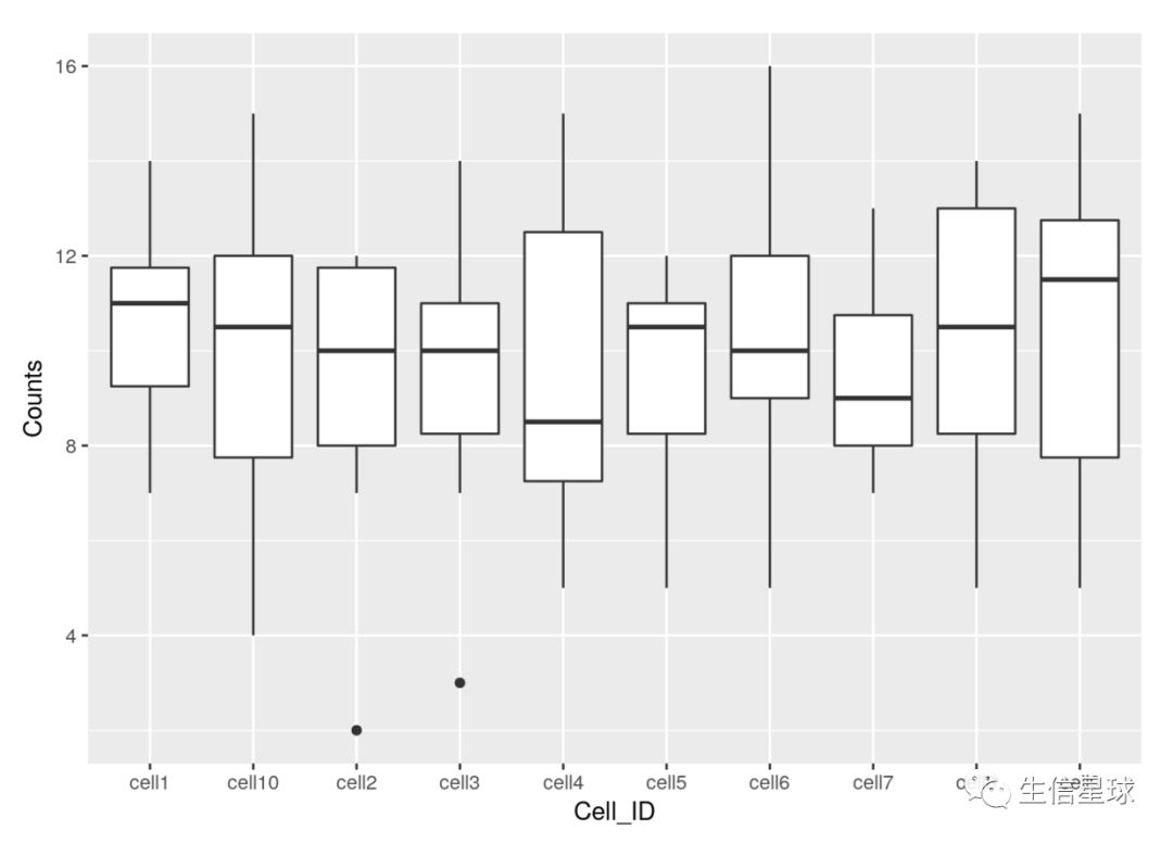
结果出来,发现没什么关系,因为是随机数据嘛,但是现在我们如果想看10组细胞间有什么差别,那么选择散点图就不好了,就用箱线图吧
**问题来了:**aes是要指定x和y的,那么十组数据怎么指定?难不成要一个一个画上去?
**注意:**这里tidy的思想就真正发挥了作用,再看一眼上面的数据,cell1~cell10,其中全是数据,是不是想到了变量少了就gather 这句话?是的,我们需要把cell变成一列,然后数据放在另一列
counts<-gather(counts, colnames(counts)[2:11], key = 'Cell_ID', value='Counts')
head(counts)
##   Gene_ids Cell_ID Counts
## 1    gene1   cell1      8
## 2    gene2   cell1     10
## 3    gene3   cell1      7
## 4    gene4   cell1     11
## 5    gene5   cell1     14
## 6    gene6   cell1     12

#然后ggplot轻松使用
ggplot(counts,aes(x=Cell_ID, y=Counts)) + geom_boxplot()