scRNA-单细胞转录组学习笔记-18-scRNA包学习Monocle2
刘小泽写于19.9.2- 第三单元第七讲:使用scRNA包学习Monocle2 笔记目的:根据生信技能树的单细胞转录组课程探索smart-seq2技术相关的分析技术 课程链接在:http://jm.grazy.cn/index/mulitcourse/detail.html?cid=53
前言
关于monocle2
目前monocle2可以直接利用Bioconductor安装:https://www.bioconductor.org/packages/release/bioc/html/monocle.html
if (!requireNamespace("BiocManager", quietly = TRUE))
    install.packages("BiocManager")

BiocManager::install("monocle")
# 安装的版本是2.12.0
关于这个scRNA包
内容在:https://github.com/jmzeng1314/scRNA_smart_seq2/blob/master/scRNA/study_scRNAseq.html
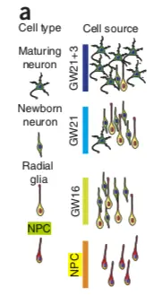
要使用scRNAseq这个R包,首先要对它进行了解,包中内置了Pollen et al. 2014 的数据集(https://www.nature.com/articles/nbt.2967),到19年8月为止,已经有446引用量了。只不过原文完整的数据是 23730 个基因, 301 个样本【这里只有130个样本文库(高覆盖度、低覆盖度各65个,并且测序深度不同】,这个包中只选取了4种细胞类型:pluripotent stem cells 分化而成的 neural progenitor cells (NPC,神经前体细胞) ,还有 GW16(radial glia,放射状胶质细胞) 、GW21(newborn neuron,新生儿神经元) 、GW21+3(maturing neuron,成熟神经元) ,它们的关系如下图(NPC和其他三类存在较大差别):
数据大小是50.6 MB,要想知道数据怎么处理的,可以看:https://hemberg-lab.github.io/scRNA.seq.datasets/human/tissues/
加载scRNA包中的数据
library(scRNAseq)
data(fluidigm)

> fluidigm
class: SummarizedExperiment
dim: 26255 130
metadata(3): sample_info clusters which_qc
assays(4): tophat_counts cufflinks_fpkm rsem_counts rsem_tpm
rownames(26255): A1BG A1BG-AS1 ... ZZEF1 ZZZ3
rowData names(0):
colnames(130): SRR1275356 SRR1274090 ... SRR1275366 SRR1275261
colData names(28): NREADS NALIGNED ... Cluster1 Cluster2
创建CellDataSet对象
=> newCellDataSet()
# 这个对象需要三个要素
# 第一个:RSEM表达矩阵(ct = count)
assay(fluidigm)  <-  assays(fluidigm)$rsem_counts
ct <- floor(assays(fluidigm)$rsem_counts)
ct[1:4,1:4]
# 第二个:临床信息
sample_ann <- as.data.frame(colData(fluidigm))
# 第三个:基因注释信息(必须包含一列是gene_short_name)
gene_ann <- data.frame(
  gene_short_name = row.names(ct),
  row.names = row.names(ct)
)
# 然后转换为AnnotatedDataFrame对象
pd <- new("AnnotatedDataFrame",
          data=sample_ann)
fd <- new("AnnotatedDataFrame",
          data=gene_ann)

# 最后构建CDS对象
sc_cds <- newCellDataSet(
  ct,
  phenoData = pd,
  featureData =fd,
  expressionFamily = negbinomial.size(),
  lowerDetectionLimit=1)
sc_cds
# CellDataSet (storageMode: environment)
# assayData: 26255 features, 130 samples
# element names: exprs
# protocolData: none
# phenoData
# sampleNames: SRR1275356 SRR1274090 ... SRR1275261 (130 total)
# varLabels: NREADS NALIGNED ... Size_Factor (29 total)
# varMetadata: labelDescription
# featureData
# featureNames: A1BG A1BG-AS1 ... ZZZ3 (26255 total)
# fvarLabels: gene_short_name
# fvarMetadata: labelDescription
# experimentData: use 'experimentData(object)'
# Annotation:
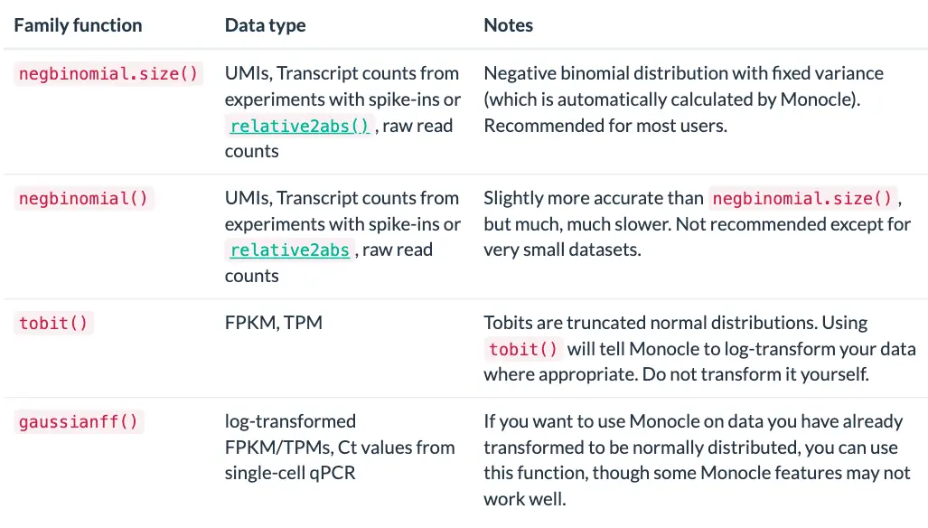
注意到构建CDS对象过程中有一个参数是:expressionFamily ,它是选择了一个数据分布,例如FPKM/TPM 值是log-正态分布的;UMIs和原始count值用负二项分布模拟的效果更好。负二项分布有两种方法,这里选用了negbinomial.size,另外一种negbinomial稍微更准确一点,但速度大打折扣,它主要针对非常小的数据集
质控过滤
=> detectGenes()
cds=sc_cds
cds ## 原始数据有: 26255 features, 130 samples
# 设置一个基因表达量的过滤阈值,结果会在cds@featureData@data中新增一列num_cells_expressed,记录这个基因在多少细胞中有表达
cds <- detectGenes(cds, min_expr = 0.1)
# 结果保存在cds@featureData@data
print(head(cds@featureData@data))
# gene_short_name num_cells_expressed
# A1BG                A1BG                  10
# A1BG-AS1        A1BG-AS1                   2
# A1CF                A1CF                   1
# A2M                  A2M                  21
# A2M-AS1          A2M-AS1                   3
# A2ML1              A2ML1                   9
在monocle版本2.12.0中,取消了fData函数(此前在2.10版本中还存在),不过在monocle3中又加了回来
如果遇到不能使用fData的情况,就可以采用备选方案:cds@featureData@data
然后可以进行基因过滤 =>subset()
expressed_genes <- row.names(subset(cds@featureData@data,
                                    num_cells_expressed >= 5))
length(expressed_genes)
## [1] 13385
cds <- cds[expressed_genes,]
还可以进行细胞层面的过滤(可选)
# 依然是:如果不支持使用pData()函数,可以使用cds@phenoData@data来获得各种细胞注释信息
print(head(cds@phenoData@data))
# 比如我们看一下细胞注释的第一个NREADS信息
tmp=pData(cds)
fivenum(tmp[,1])
## [1]    91616   232899   892209  8130850 14477100

# 如果要过滤细胞,其实也是利用subset函数,不过这里不会对细胞过滤
valid_cells <- row.names(cds@phenoData@data)
cds <- cds[,valid_cells]
cds
## CellDataSet (storageMode: environment)
## assayData: 13385 features, 130 samples
##   element names: exprs
## protocolData: none
## phenoData
##   sampleNames: SRR1275356 SRR1274090 ... SRR1275261 (130 total)
##   varLabels: NREADS NALIGNED ... num_genes_expressed (30 total)
##   varMetadata: labelDescription
## featureData
##   featureNames: A1BG A2M ... ZZZ3 (13385 total)
##   fvarLabels: gene_short_name num_cells_expressed
##   fvarMetadata: labelDescription
## experimentData: use 'experimentData(object)'
## Annotation:
聚类
在monocle3中,聚类使用的是
cluster_cells(),利用Louvain community detection的非监督聚类方法,结果保存在cds@clusters$UMAP$clusters
不使用marker基因聚类
使用函数clusterCells(),根据整体的表达量对细胞进行分组。例如,细胞表达了大量的与成肌细胞相关的基因,但就是没有成肌细胞的marker–MYF5 ,我们依然可以判断这个细胞属于成肌细胞。
step1:dispersionTable()
首先就是判断使用哪些基因进行细胞分群。当然,可以使用全部基因,但这会掺杂很多表达量不高而检测不出来的基因,反而会增加噪音。挑有差异的,挑表达量不太低的
cds <- estimateSizeFactors(cds)
cds <- estimateDispersions(cds)
disp_table <- dispersionTable(cds) # 挑有差异的
unsup_clustering_genes <- subset(disp_table, mean_expression >= 0.1) # 挑表达量不太低的
cds <- setOrderingFilter(cds, unsup_clustering_genes$gene_id) # 准备聚类基因名单
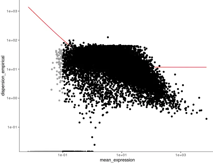
plot_ordering_genes(cds)
# 图中黑色的点就是被标记出来一会要进行聚类的基因
step2:plot_pc_variance_explained()
然后选一下主成分
plot_pc_variance_explained(cds, return_all = F) # norm_method='log'

step3:
根据上面👆的图,选择合适的主成分数量(这个很主观,可以多试几次),这里选前6个成分(大概在第一个拐点处)
# 进行降维
cds <- reduceDimension(cds, max_components = 2, num_dim = 6,
reduction_method = 'tSNE', verbose = T)
# 进行聚类
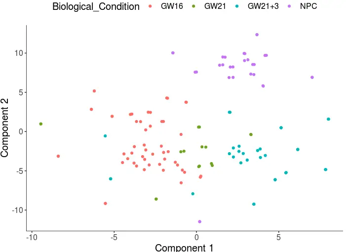
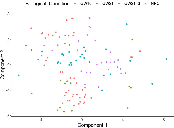
cds <- clusterCells(cds, num_clusters = 4)
# Distance cutoff calculated to 0.5225779
plot_cell_clusters(cds, 1, 2, color = "Biological_Condition")

> table(cds@phenoData@data$Biological_Condition)

  GW16   GW21 GW21+3    NPC
    52     16     32     30
需要注意的是,使用的主成分数量会影响结果
前面使用了6个主成分,分的还不错。现在假设使用前16个主成分:
cds <- reduceDimension(cds, max_components = 2, num_dim = 16,
                       reduction_method = 'tSNE', verbose = T)
cds <- clusterCells(cds, num_clusters = 4)
plot_cell_clusters(cds, 1, 2, color = "Biological_Condition")
以下是测试代码!
除此以外,如果有批次效应等干扰因素,也可以在降维(reduceDimension())的过程中进行排除:
if(F){
  cds <- reduceDimension(cds, max_components = 2, num_dim = 6,
                         reduction_method = 'tSNE',
                         residualModelFormulaStr = "~Biological_Condition + num_genes_expressed",
                         verbose = T)
  cds <- clusterCells(cds, num_clusters = 4)
  plot_cell_clusters(cds, 1, 2, color = "Biological_Condition")
}
# 可以看到,去掉本来的生物学意义后,最后细胞是会被打散的。所以residualModelFormulaStr这个东西的目的就是磨平它参数包含的差异
但是,如果是去除其他的效应:
# 如果去除生物意义以外的效应
  cds <- reduceDimension(cds, max_components = 2, num_dim = 6,
                         reduction_method = 'tSNE',
                         residualModelFormulaStr = "~NREADS + num_genes_expressed",
                         verbose = T)
  cds <- clusterCells(cds, num_clusters = 4)
  plot_cell_clusters(cds, 1, 2, color = "Biological_Condition")

关于处理批次效应:例如在芯片数据中经常会利用SVA的combat函数。 磨平批次效应实际上就是去掉各个组的前几个主成分
差异分析
=> differentialGeneTest()
start=Sys.time()
diff_test_res <- differentialGeneTest(cds,
                                      fullModelFormulaStr = "~Biological_Condition")
end=Sys.time()
end-start
# 运行时间在几分钟至十几分钟不等
然后得到差异基因
sig_genes <- subset(diff_test_res, qval < 0.1)
> head(sig_genes[,c("gene_short_name", "pval", "qval")] )
      gene_short_name         pval         qval
A1BG             A1BG 4.112065e-04 1.460722e-03
A2M               A2M 4.251744e-08 4.266086e-07
AACS             AACS 2.881832e-03 8.275761e-03
AADAT           AADAT 1.069794e-02 2.621123e-02
AAGAB           AAGAB 1.156771e-07 1.021331e-06
AAMP             AAMP 7.626789e-05 3.243869e-04
作图(注意要将基因名变成character)
cg=as.character(head(sig_genes$gene_short_name))
# 普通图
plot_genes_jitter(cds[cg,],
                  grouping = "Biological_Condition", ncol= 2)
# 还能上色
plot_genes_jitter(cds[cg,],
                  grouping = "Biological_Condition",
                  color_by = "Biological_Condition",
                  nrow= 3,
                  ncol = NULL )

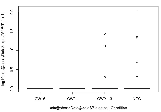
我们自己也可以根据某个基因的表达量差异和分组信息进行作图(就以A1BG为例):
# 以A1BG为例
boxplot(log10(cds@assayData$exprs["A1BG",]+1) ~ cds@phenoData@data$Biological_Condition)
推断发育轨迹
**三步走:**从差异分析结果选合适基因=》降维=》细胞排序
step1: 选合适基因
ordering_genes <- row.names (subset(diff_test_res, qval < 0.01))
cds <- setOrderingFilter(cds, ordering_genes)
plot_ordering_genes(cds)
step2: 降维
# 默认使用DDRTree的方法
cds <- reduceDimension(cds, max_components = 2,
                            method = 'DDRTree')
step3: 细胞排序
cds <- orderCells(cds)
最后可视化
plot_cell_trajectory(cds, color_by = "Biological_Condition")

这个图就可以看到细胞的发展过程
另外,plot_genes_in_pseudotime 可以对基因在不同细胞中的表达量变化进行绘图
plot_genes_in_pseudotime(cds[cg,],
                         color_by = "Biological_Condition")
