scRNA-10X免疫治疗学习笔记-5-差异分析及可视化
刘小泽写于19.10.17 笔记目的:根据生信技能树的单细胞转录组课程探索10X Genomics技术相关的分析 课程链接在:http://jm.grazy.cn/index/mulitcourse/detail.html?cid=55 第二单元第9讲:细胞亚群之间的差异分析
前言
这次的任务是模仿原文的:
第五张:比较两种CD8+细胞差异
在分群结果可以看到,CD8+主要分成了两群,一个是红色的(170个CD8+ cytotoxic T cells,即 细胞毒性T细胞),一个是浅蓝色的(429个CD8+ effector T cells,即 效应T细胞)
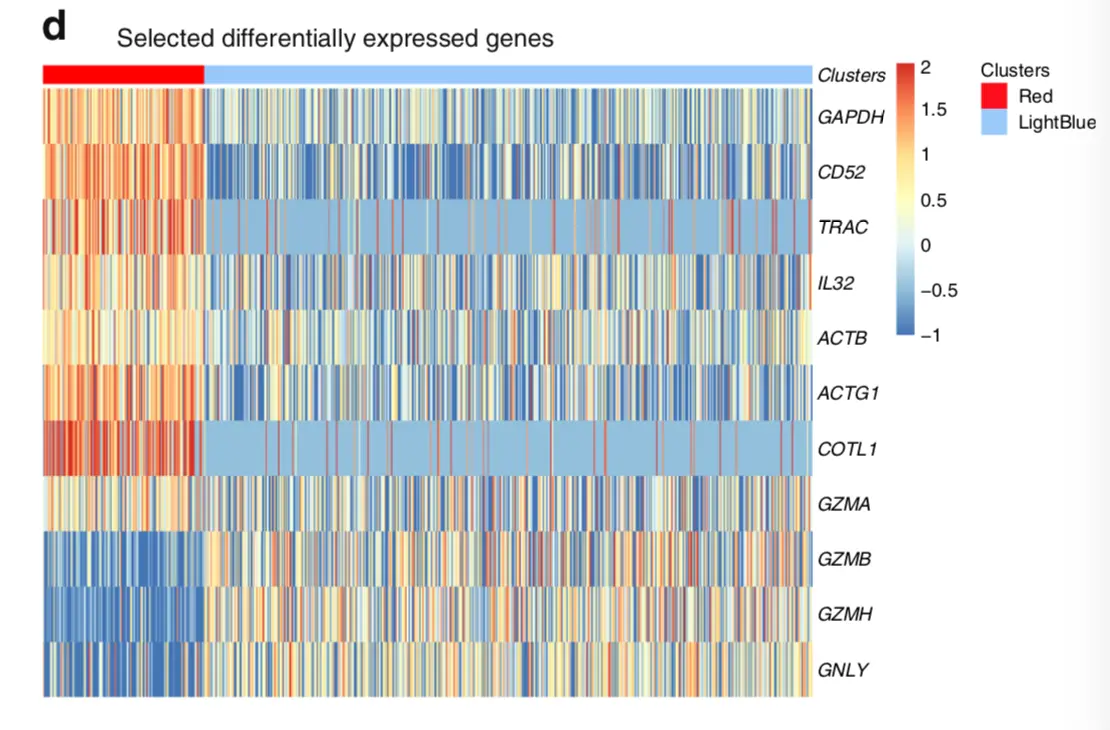
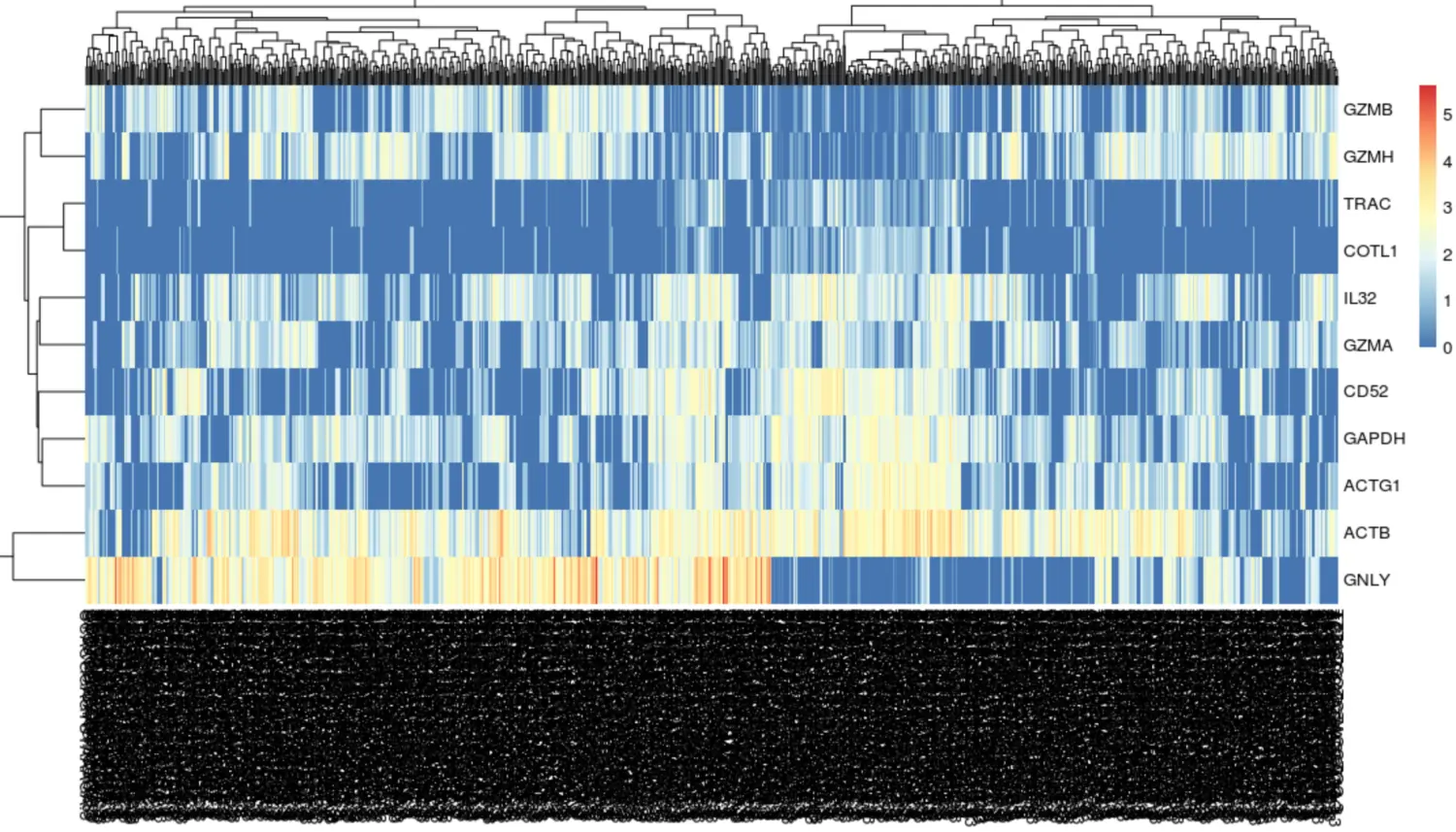
【图片注释:Heat map of selected significantly differentially expressed genes comparing CD8+ T cells in the red activated cluster (n = 170) to those in the blue effector/EM cluster (n = 429) at response (day + 376) 】
首先进行差异分析
准备数据
=> SubsetData()取子集
既然是分析的day +376数据,那么就先把这一小部分数据提取出来:
rm(list = ls())
options(warn=-1)
suppressMessages(library(Seurat))
load('./patient1.PBMC.output.Rdata')

PBMC_RespD376 = SubsetData(PBMC,TimePoints =='PBMC_RespD376')
> table(PBMC_RespD376@ident)

  0   1   2   3   4   5   6   7   8   9  10  11  12
800 433 555 677 636 516 119 324 204 200 170  11  39
然后这个图是分析了红色和浅蓝色的两群,结合之前得到的分群结果,红色是第10群,浅蓝色是第4群
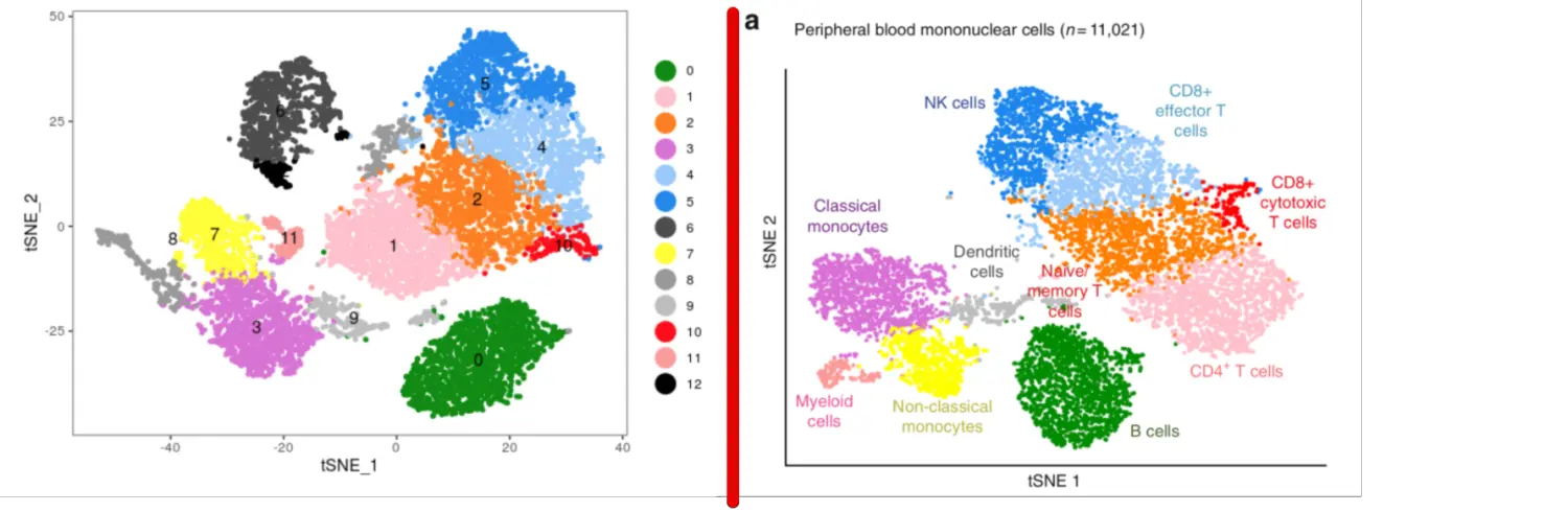
于是再用这个函数提取出来第4、10群
PBMC_RespD376_for_DEG = SubsetData(PBMC_RespD376,
                                   PBMC_RespD376@ident %in% c(4,10))
利用monocle V2构建对象
=> newCellDataSet()
我们需要三样东西:表达矩阵、细胞信息、基因信息
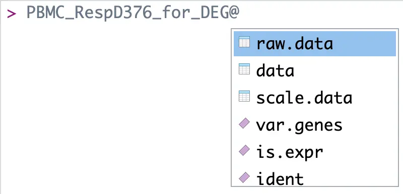
首先来看表达矩阵:上面取到的PBMC_RespD376_for_DEG中包含了多个数据接口,单是表达矩阵相关就有三个
关于这三者的不同:
We view
object@raw.dataas a storage slot for the non-normalized data, upon which we perform normalization and returnobject@data.(来自:https://github.com/satijalab/seurat/issues/351)也就是说,raw.data是最原始的矩阵,data是归一化之后的,scale.data是标准化后的(一般是z-score处理)
data:The normalized expression matrix (log-scale)scale.data:scaled (default is z-scoring each gene) expression matrix; used for dimmensional reduction and heatmap visualization(来自: seurat的各个接口含义)
我们使用log处理过的归一化表达矩阵
count_matrix=PBMC_RespD376_for_DEG@data
> dim(count_matrix)
[1] 17712   806
然后,看细胞信息
# 细胞分群信息
cluster=PBMC_RespD376_for_DEG@ident
> table(cluster)
cluster
  4  10
636 170
# 细胞名称(barcode名称)
names(count_matrix)
最后是基因信息
gene_annotation <- as.data.frame(rownames(count_matrix))
万事俱备,开始monocle
library(monocle)
> packageVersion('monocle')
[1] ‘2.12.0’
# 1.表达矩阵
expr_matrix <- as.matrix(count_matrix)
# 2.细胞信息
sample_ann <- data.frame(cells=names(count_matrix),
cellType=cluster)
rownames(sample_ann)<- names(count_matrix)
# 3.基因信息
gene_ann <- as.data.frame(rownames(count_matrix))
rownames(gene_ann)<- rownames(count_matrix)
colnames(gene_ann)<- "genes"
# 然后转换为AnnotatedDataFrame对象
pd <- new("AnnotatedDataFrame",
data=sample_ann)
fd <- new("AnnotatedDataFrame",
data=gene_ann)
# 最后构建CDS对象
sc_cds <- newCellDataSet(
expr_matrix,
phenoData = pd,
featureData =fd,
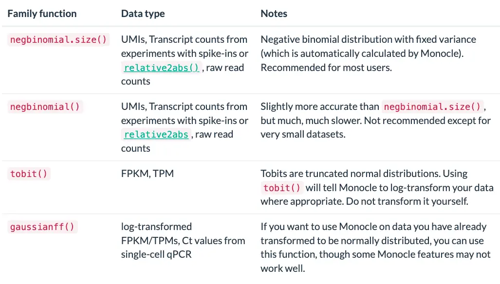
expressionFamily = negbinomial.size(),
lowerDetectionLimit=1)
关于其中的参数expressionFamily :负二项分布有两种方法,这里选用了negbinomial.size ; 另外一种negbinomial稍微更准确一点,但速度大打折扣,它主要针对非常小的数据集
monocle V2质控过滤
=> detectGenes() + subset()
cds=sc_cds
cds <- detectGenes(cds, min_expr = 0.1)
# 结果保存在cds@featureData@data
> print(head(cds@featureData@data))
                      genes num_cells_expressed
RP11-34P13.7   RP11-34P13.7                   0
FO538757.2       FO538757.2                  20
AP006222.2       AP006222.2                  11
RP4-669L17.10 RP4-669L17.10                   0
RP11-206L10.9 RP11-206L10.9                   5
LINC00115         LINC00115                   0
在monocle版本2.12.0中,取消了fData函数(此前在2.10版本中还存在)。如果遇到不能使用fData的情况,就可以采用备选方案:cds@featureData@data
然后进行基因过滤 =>subset()
expressed_genes <- row.names(subset(cds@featureData@data,
                                    num_cells_expressed >= 5))

> length(expressed_genes)
[1] 12273

cds <- cds[expressed_genes,]
monocle V2 聚类
step1:dispersionTable() 目的是判断使用哪些基因进行细胞分群
当然可以使用全部基因,但这会掺杂很多表达量不高而检测不出来的基因,反而会增加噪音。最好是挑有差异的,挑表达量不太低的
cds <- estimateSizeFactors(cds)
cds <- estimateDispersions(cds)
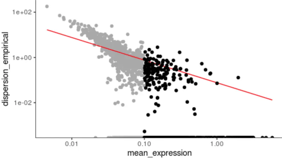
disp_table <- dispersionTable(cds) # 挑有差异的
unsup_clustering_genes <- subset(disp_table, mean_expression >= 0.1) # 挑表达量不太低的
cds <- setOrderingFilter(cds, unsup_clustering_genes$gene_id) # 准备聚类基因名单
plot_ordering_genes(cds)
# 图中黑色的点就是被标记出来一会要进行聚类的基因
[可省略]step2:plot_pc_variance_explained() 选一下主成分
plot_pc_variance_explained(cds, return_all = F) # norm_method='log'
step3: 聚类
# 进行降维
cds <- reduceDimension(cds, max_components = 2, num_dim = 6,
reduction_method = 'tSNE', verbose = T)
# 进行聚类
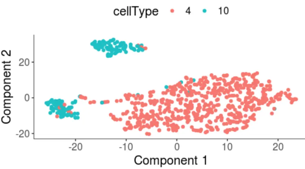
cds <- clusterCells(cds, num_clusters = 4)
# Distance cutoff calculated to 1.812595
plot_cell_clusters(cds, 1, 2, color = "cellType")
monocle V2 差异分析
=> differentialGeneTest()
# 这个过程比较慢!
start=Sys.time()
diff_test_res <- differentialGeneTest(cds,
                                      fullModelFormulaStr = "~cellType")
end=Sys.time()
end-start
# Time difference of 5.729718 mins
然后得到差异基因
sig_genes <- subset(diff_test_res, qval < 0.1)
> nrow(sig_genes)
[1] 635
# 最后会得到635个差异基因

> head(sig_genes[,c("genes", "pval", "qval")] )
            genes         pval        qval
ISG15       ISG15 1.493486e-03 0.040823046
CCNL2       CCNL2 2.228521e-03 0.055590716
MIB2         MIB2 4.954659e-05 0.002523176
MMP23B     MMP23B 1.009464e-04 0.004657577
TNFRSF25 TNFRSF25 1.608900e-04 0.006785583
CAMTA1     CAMTA1 4.339489e-03 0.090162380
进行热图可视化
文章使用的基因如下(也就是第一张图中显示的)
htmapGenes=c(
  'GAPDH','CD52','TRAC','IL32','ACTB','ACTG1','COTL1',
  'GZMA','GZMB','GZMH','GNLY'
)
# 看到作者挑选的这些基因也都出现在我们自己分析的结果中
> htmapGenes %in% rownames(sig_genes)
 [1] TRUE TRUE TRUE TRUE TRUE TRUE TRUE TRUE TRUE TRUE TRUE
下面开始画图
先画一个最最最原始的
library(pheatmap)
dat=count_matrix[htmapGenes,]
pheatmap(dat)
需要修改的地方:列名(barcode)不需要、聚类不需要、数据需要z-score
再来一版
n=t(scale(t(dat)))
# 规定上下限(和原文保持一致)
n[n>2]=2
n[n< -1]= -1
> n[1:4,1:4]
      AAACCTGCAACGATGG.3 AAACCTGGTCTCCATC.3 AAACGGGAGCTCCTTC.3
GAPDH         -1.0000000        -0.06057709        -0.37324949
CD52           0.6676167         0.31653833         0.04253204
TRAC           0.7272507         0.63277670        -0.51581312
IL32          -1.0000000         0.42064114        -0.16143114
      AAAGCAATCATATCGG.3
GAPDH         -1.0000000
CD52          -1.0000000
TRAC          -0.5158131
IL32           0.1548693

# 加上细胞归属注释(ac = annotation column),去掉列名和聚类
ac=data.frame(group=cluster)
rownames(ac)=colnames(n)

pheatmap(n,annotation_col = ac,
         show_colnames =F,
         show_rownames = T,
         cluster_cols = F,
         cluster_rows = F)
