scRNA-小鼠发育学习笔记-1-前言及上游介绍
刘小泽写于19.10.23 笔记目的:根据生信技能树的单细胞转录组课程探索Smartseq2技术及发育相关的分析 课程链接在:http://jm.grazy.cn/index/mulitcourse/detail.html?cid=55 这次会介绍文章的两张主图,还有上游分析,算是引言部分。对应视频第三单元1-4讲
前言
文章方法思路
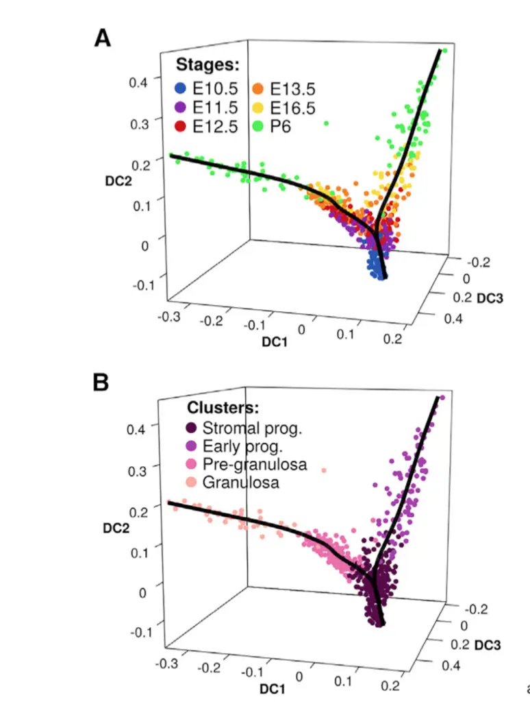
为了研究卵巢发育过程中体细胞谱系特征,作者结合Fluidigm C1分选和smartseq2建库,在Tg(Nr5a1-GFP)转基因小鼠性腺分化的6个时期(E10.5, E11.5, E12.5, E13.5, E16.5, and post-natalday6)提取了663个细胞( GSE119766),然后使用Hiseq2000 进行双端100bp测序,每个细胞测10M reads。
经过比对、定量得到表达矩阵,然后对细胞进行过滤,最后剩下563个。进行PCA,用
Jackstraw提取了最显著的几个主成分,并用FactoMineR进行HCPC 聚类,使用Rtsne进行tSNE,然后分群,得到了4个胚胎发育时期(C1到C4),之后对标记基因进行可视化(包括等高线图和热图,使用了自己包装的大量代码)。然后对C1-C4每个群进行差异分析(使用monocle2),差异基因进行功能注释(使用clusterProfiler和PANTHER)
根据高变化基因进行细胞谱系推断,利用
diffusion map的Destiny和Slingshot。后来谱系发育基因进行了可视化、聚类和注释
综上,文章得到了6个发育时期、4群细胞、2个发育轨迹这三种细胞属性
重要的信息如下:
分群信息(对应课程下游分析之第5、6讲)
标记基因可视化(对应课程下游分析之第7、8讲)
差异分析及注释(对应课程下游分析之第9、10讲)
比较不同的差异分析方法,如monocle、ROST(对应课程下游分析之第11讲)
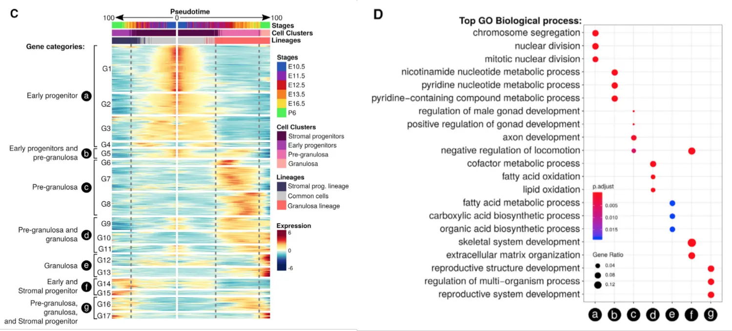
谱系推断(对应课程下游分析之第12讲)
谱系发育基因可视化(对应课程下游分析之第13讲)
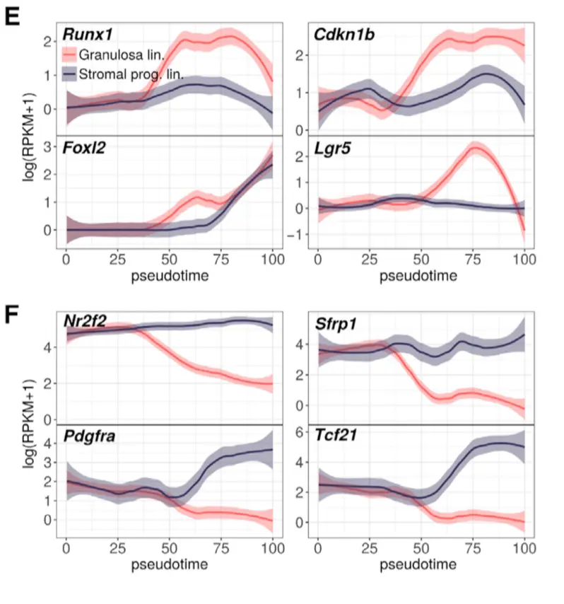
谱系发育基因聚类和注释(对应课程下游分析之第14讲)
上游分析
将会对应课程的全部上游分析第1-4讲 这部分和转录组分析很相似,所以也是简单带过
smartseq2得到的文件和10X的不一样,10X的数据虽然也有R1、R2两个数据,但第一个存储的是barcode和UMI信息,而只有第二个才是真正的测序信息,也就是单端测序;而smartseq2得到的两个R1、R2都是测序信息,于是它的操作和我们常规bulk转录组是类似的。可以用hisat2+featureCounts进行操作;或者如果不想比对的话,也可以用salmon进行操作
配置conda
# 安装conda
wget https://mirrors.tuna.tsinghua.edu.cn/anaconda/miniconda/Miniconda3-latest-Linux-x86_64.sh
bash Miniconda3-latest-Linux-x86_64.sh
# 激活
source ~/.bashrc

# 添加镜像
conda config --add channels r
conda config --add channels conda-forge
conda config --add channels bioconda
conda config --add channels https://mirrors.tuna.tsinghua.edu.cn/anaconda/pkgs/free
conda config --add channels https://mirrors.tuna.tsinghua.edu.cn/anaconda/cloud/conda-forge
conda config --add channels https://mirrors.tuna.tsinghua.edu.cn/anaconda/cloud/bioconda
conda config --set show_channel_urls yes

# 创建环境
conda  create -n rna  python=2
conda activate rna
conda install -y  sra-tools trim-galore fastqc multiqc hisat2 samtools subread salmon qualimap

#注销当前的rna环境
# conda deactivate
下载数据
XX全部的数据比较大,数据在:https://www.ncbi.nlm.nih.gov/Traces/study/?acc=PRJNA490198&o=acc_s%3Aa
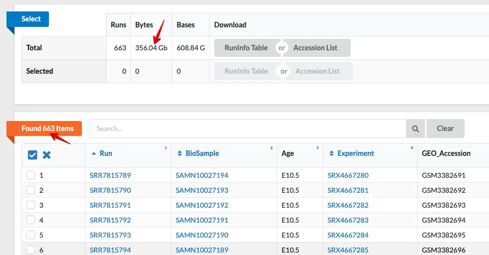
因此简单下几个体验一下就好,我这里选取了这些:
# wkd=/YOUR_PATH/
# cd $wkd/sra
# 这些数据全部都放在了EBI,而不是NCBI
SRR7815790
SRR7815850
SRR7815870
SRR7815890
SRR7815910
SRR7815960
SRR7815980
SRR7816020
SRR7816100
SRR7816120
SRR7816130
SRR7816140
SRR7816160
如果prefetch + ascp可以用的话,那是最好,因为那是最省事的下载办法,而且不用管SRA数据是来自欧洲的EBI还是美国的NCBI。如果出现了使用https下载方式,而非快速的fasp下载,可以看这个:
来吧,加速你的下载
需要注意EBI和NCBI的SRA数据存储结构有些区别:
NCBI的文件存在
ftp://ftp.ncbi.nlm.nih.gov/sra/sra-instant/reads/ByRun/sra/SRR/EBI文件存在
ftp://ftp.sra.ebi.ac.uk/vol1/srr例如要下载SRR7815792.sra,它就是
ftp://ftp.sra.ebi.ac.uk/vol1/srr/SRR781/002/SRR7815792,倒数第二个位置的002是和SRR ID的最后一个数字对应的,另外EBI下载的名称没有后缀.sra
sra2fq
wkd=/YOUR_PATH/
ls $wkd/sra/SRR* | while read i;do \
	(fastq-dump --gzip --split-3 -A `basename $i` -O $wkd/rawdata $i &);done
下载参考数据
# 从Gencode下载参考基因组
wget ftp://ftp.ebi.ac.uk/pub/databases/gencode/Gencode_mouse/release_M23/GRCm38.primary_assembly.genome.fa.gz
# 从Gencode下载参考转录组
wget ftp://ftp.ebi.ac.uk/pub/databases/gencode/Gencode_mouse/release_M23/gencode.vM23.transcripts.fa.gz
# 下载GTF文件
wget ftp://ftp.ebi.ac.uk/pub/databases/gencode/Gencode_mouse/release_M23/gencode.vM23.annotation.gtf.gz
基于比对的hisat2流程
构建索引
ref=$wkd/reference/mm10.fasta
hisat2-build -p 40 $ref hisat.mm10
# 历时:00:14:39
如果不想自己构建索引,可以直接下载hisat官网数据
wget ftp://ftp.ccb.jhu.edu/pub/infphilo/hisat2/data/mm10.tar.gz
比对过程
# 以其中SRR7815790为例
index=$wkd/hisat/hisat.mm10
hisat2 -p 10 -x $index -1 SRR7815790_1.fastq.gz -2 SRR7815790_2.fastq.gz  --new-summary -S SRR7815790_hisat.sam

samtools sort -O bam -@ 10  -o SRR7815790_hisat.bam SRR7815790_hisat.sam

samtools index -@ 10 -b SRR7815790_hisat.bam
比对结果
# 看到有一个细胞(SRR7816020)质量不好,后面需要去除
SRR7815790.hisat.log:	Overall alignment rate: 90.14%
SRR7815850.hisat.log:	Overall alignment rate: 87.49%
SRR7815870.hisat.log:	Overall alignment rate: 87.39%
SRR7815890.hisat.log:	Overall alignment rate: 90.08%
SRR7815910.hisat.log:	Overall alignment rate: 90.32%
SRR7815960.hisat.log:	Overall alignment rate: 91.73%
SRR7815980.hisat.log:	Overall alignment rate: 86.01%
SRR7816020.hisat.log:	Overall alignment rate: 61.82%
SRR7816100.hisat.log:	Overall alignment rate: 88.14%
SRR7816120.hisat.log:	Overall alignment rate: 90.21%
SRR7816130.hisat.log:	Overall alignment rate: 87.30%
SRR7816140.hisat.log:	Overall alignment rate: 89.59%
SRR7816160.hisat.log:	Overall alignment rate: 84.33%
SRR7815790.hisat.log:Execution time for SRR7815790 hisat and sam2bam : 115.350829 seconds
SRR7815850.hisat.log:Execution time for SRR7815850 hisat and sam2bam : 149.416581 seconds
SRR7815870.hisat.log:Execution time for SRR7815870 hisat and sam2bam : 218.976666 seconds
SRR7815890.hisat.log:Execution time for SRR7815890 hisat and sam2bam : 168.738353 seconds
SRR7815910.hisat.log:Execution time for SRR7815910 hisat and sam2bam : 214.020996 seconds
SRR7815960.hisat.log:Execution time for SRR7815960 hisat and sam2bam : 169.597353 seconds
SRR7815980.hisat.log:Execution time for SRR7815980 hisat and sam2bam : 146.707250 seconds
SRR7816020.hisat.log:Execution time for SRR7816020 hisat and sam2bam : 3.484966 seconds
SRR7816100.hisat.log:Execution time for SRR7816100 hisat and sam2bam : 131.300152 seconds
SRR7816120.hisat.log:Execution time for SRR7816120 hisat and sam2bam : 133.382700 seconds
SRR7816130.hisat.log:Execution time for SRR7816130 hisat and sam2bam : 124.014219 seconds
SRR7816140.hisat.log:Execution time for SRR7816140 hisat and sam2bam : 166.373111 seconds
SRR7816160.hisat.log:Execution time for SRR7816160 hisat and sam2bam : 209.587995 seconds
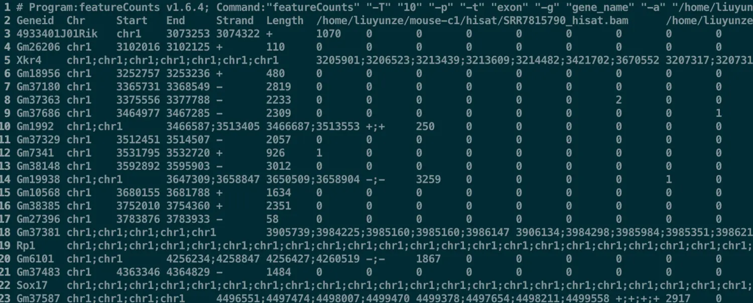
定量
gtf=$wkd/reference/gencode.vM23.annotation.gtf
featureCounts  -T 10 -p -t exon -g gene_name -a $gtf -o $wkd/hisat/count/hisat2_counts.txt $wkd/hisat/*.bam 1>featureCounts.log 2>&1
不基于比对的salmon流程
salmon需要对转录本构建索引。因此只能使用参考转录组,而不能使用基因组
构建索引
ref=$wkd/reference/gencode.vM23.transcripts.fa
salmon index -t $ref -i salmon.mm10
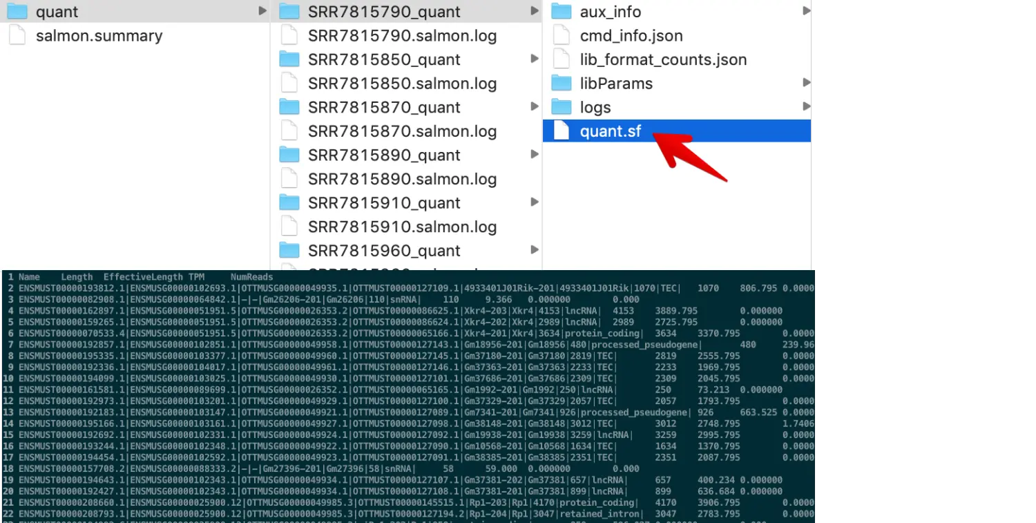
定量
# 以其中SRR7815790为例
index=$wkd/salmon/salmon.mm10
salmon quant -i $index -l A --validateMappings \
		-1 SRR7815790_1.fastq.gz -2 SRR7815790_2.fastq.gz \
		-p 10 -o SRR7815790_quant 1>SRR7815790.salmon.log 2>&1
运行速度的确很快
SRR7815790.salmon.log:Execution time for SRR7815790 salmon : 36.016640 seconds
SRR7815850.salmon.log:Execution time for SRR7815850 salmon : 54.478129 seconds
SRR7815870.salmon.log:Execution time for SRR7815870 salmon : 76.499805 seconds
SRR7815890.salmon.log:Execution time for SRR7815890 salmon : 58.166234 seconds
SRR7815910.salmon.log:Execution time for SRR7815910 salmon : 56.277339 seconds
SRR7815960.salmon.log:Execution time for SRR7815960 salmon : 52.918936 seconds
SRR7815980.salmon.log:Execution time for SRR7815980 salmon : 47.993982 seconds
SRR7816020.salmon.log:Execution time for SRR7816020 salmon : 8.981974 seconds
SRR7816100.salmon.log:Execution time for SRR7816100 salmon : 40.505802 seconds
SRR7816120.salmon.log:Execution time for SRR7816120 salmon : 52.856553 seconds
SRR7816130.salmon.log:Execution time for SRR7816130 salmon : 38.405255 seconds
SRR7816140.salmon.log:Execution time for SRR7816140 salmon : 53.823648 seconds
SRR7816160.salmon.log:Execution time for SRR7816160 salmon : 75.848338 seconds
Salmon的结果和Hisat的不同,它的每个数据都是独立的文件夹,其中quant.sf 就是每个样本的定量结果
对于salmon的定量结果,需要用到R里面的tximport 导入
tximport函数主要需要两个参数:定量文件files和转录本与基因名的对应文件tx2gene
rm(list = ls())
options(stringsAsFactors = F)

####################
# 配置files路径
####################
dir <- file.path(getwd(),'quant/')
dir
files <- list.files(pattern = '*sf',dir,recursive = T)
files <- file.path(dir,files)
all(file.exists(files))

####################
# 配置tx2gene
####################
# https://support.bioconductor.org/p/101156/
# BiocManager::install("EnsDb.Mmusculus.v79")
# 如何构建?
if(F){
  library(EnsDb.Mmusculus.v79)
  txdf <- transcripts(EnsDb.Mmusculus.v79, return.type="DataFrame")
  mm10_tx2gene <- as.data.frame(txdf[,c("tx_id", "gene_id")])
  head(mm10_tx2gene)
  write.csv(mm10_tx2gene,file = 'mm10_tx2gene.csv')
}
tx2_gene_file <- 'mm10_tx2gene.csv'
tx2gene <- read.csv(tx2_gene_file,row.names = 1)
head(tx2gene)

####################
# 开始整合
####################
library(tximport)
library(readr)
txi <- tximport(files, type = "salmon", tx2gene = tx2gene,ignoreTxVersion = T)
names(txi)
head(txi$length)
head(txi$counts)
# 发现目前counts的列名还没有指定

####################
# 添加列名
####################
# 获取导入文件名称的ID,如SRR7815870
library(stringr)
# 先得到SRRxxxx_quant这一部分
n1 <- sapply(strsplit(files,'\\/'), function(x)x[12])
# 再得到SRRxxxx这一部分
n2 <- sapply(strsplit(n1,'_'), function(x)x[1])

colnames(txi$counts) <- n2
head(txi$counts)


####################
# 操作新得到的表达矩阵
####################
salmon_expr <- txi$counts
# 表达量取整
salmon_expr <- apply(salmon_expr, 2, as.integer)
head(salmon_expr)
# 添加行名
rownames(salmon_expr) <- rownames(txi$counts)
dim(salmon_expr)

save(salmon_expr,file = 'salmon-aggr.Rdata')
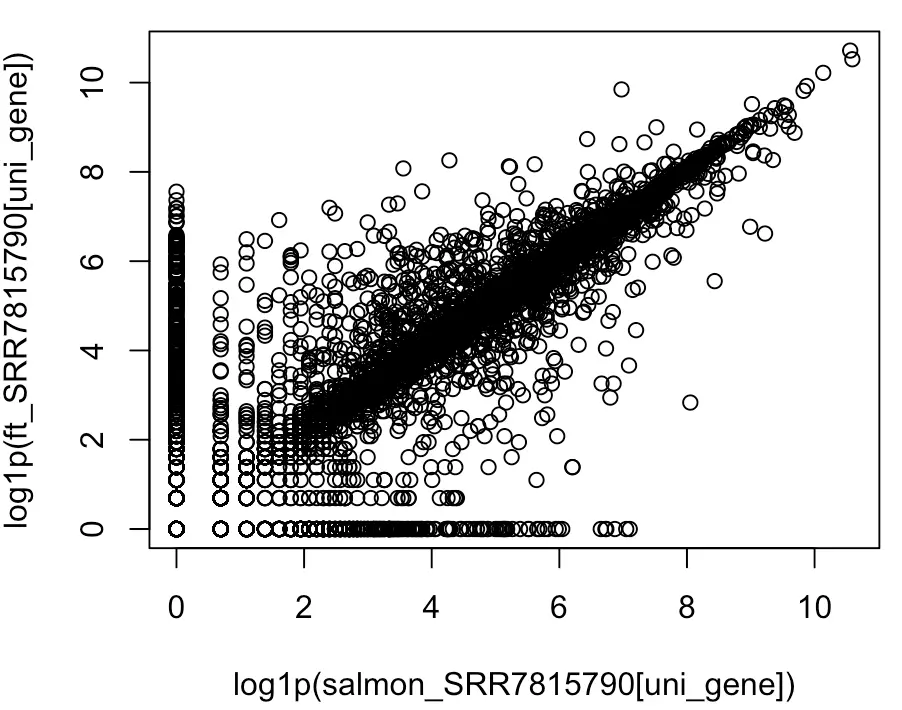
好,现在有了salmon和featureCounts两种方法得到的矩阵,就可以来比较一下
rm(list = ls())
options(stringsAsFactors = F)
load('salmon-aggr.Rdata')
dim(salmon_expr)
colnames(salmon_expr)
salmon_expr[1:3,1:3]

# 为了方便比较,我们选第一个样本SRR7815790
salmon_SRR7815790 <- salmon_expr[,1]
names(salmon_SRR7815790) <- rownames(salmon_expr)

###########################
# 然后找featureCounts结果
###########################
ft <- read.table('../hisat/hisat2_counts.txt',row.names = 1,comment.char = '#',header = T)
ft[1:4,1:4]
colnames(ft)
# 两种取子集的方法,grep返回结果的序号;grepl返回逻辑值
ft_SRR7815790 <-  ft[,grep(colnames(salmon_expr)[1], colnames(ft))]
ft_SRR7815790 <-  ft[,grepl(colnames(salmon_expr)[1], colnames(ft))]

names(ft_SRR7815790) <- rownames(ft)

###########################
# 取salmon和featureCounts公共基因
###########################
# salmon使用的Ensembl基因,而featureCounts得到的是Symbol基因
# 先进行基因名转换
library(org.Mm.eg.db)
columns(org.Mm.eg.db)
gene_tr <- clusterProfiler::bitr(names(salmon_SRR7815790),
                      "ENSEMBL","SYMBOL",
                      org.Mm.eg.db)
# 要找salmon在gene_tr中的对应位置,然后取gene_tr的第二列symbol,因此match中把salmon放第一个位置
names(salmon_SRR7815790) <- gene_tr[match(names(salmon_SRR7815790),gene_tr$ENSEMBL),2]

# 找共有基因
uni_gene <- intersect(names(salmon_SRR7815790),names(ft_SRR7815790))
length(uni_gene)

plot(log1p(salmon_SRR7815790[uni_gene]),
     log1p(ft_SRR7815790[uni_gene]))
结论就是:有些基因用不同的流程检测效果是不一样的,使用不同的参考数据得到的结果也是有区别的,但整体上一致