scRNA-几个scRNA找高变异基因(HVGs)的方法
刘小泽写于19.9.10
高变异基因就是highly variable features(HVGs),就是在细胞与细胞间进行比较,选择表达量差别最大的
1. Seurat
参考:https://satijalab.org/seurat/v3.0/pbmc3k_tutorial.html
利用FindVariableFeatures函数,会计算一个mean-variance结果,也就是给出表达量均值和方差的关系并且得到top variable features
计算方法主要有三种:
- vst(默认):首先利用loess对 log(variance) 和log(mean) 拟合一条直线,然后利用观测均值和期望方差对基因表达量进行标准化,最后根据保留最大的标准化的表达量计算方差
- mean.var.plot: 首先利用mean.function和 dispersion.function分别计算每个基因的平均表达量和离散情况,然后根据平均表达量将基因们分散到一定数量(默认是20个)的小区间(bin)中,并且计算每个bin中z-score
- dispersion(最直接):挑选最高离差值的基因
例如:使用Seurat 版本3
# V3 代码来自官方教程https://satijalab.org/seurat/v3.0/pbmc3k_tutorial.html
pbmc <- FindVariableFeatures(pbmc, selection.method = "vst", nfeatures = 2000)
top10 <- head(VariableFeatures(pbmc), 10)

# 分别绘制带基因名和不带基因名的
plot1 <- VariableFeaturePlot(pbmc)
plot2 <- LabelPoints(plot = plot1, points = top10, repel = TRUE)
CombinePlots(plots = list(plot1, plot2))

使用Seurat版本2
# V2
pbmc <- FindVariableGenes(object = pbmc,
                         mean.function = ExpMean,
                         dispersion.function = LogVMR )
length( pbmc@var.genes)
# 默认值是:x.low.cutoff = 0.1, x.high.cutoff = 8, y.cutoff = 1,就是说取log后的平均表达量(x轴)介于0.1-8之间的;分散程度(y轴,即标准差)至少为1的
- V3计算
mean.function和FastLogVMR均采用了加速的FastExpMean、FastLogVMR模式 - V3横坐标范围设定参数改成:
mean.cutoff,整合了原来V2的x.low.cutoff + x.high.cutoff;纵坐标改成:dispersion.cutoff,替代了原来V2的y.cutoff - V3默认选择2000个差异基因,检查方法也不同(V3用
VariableFeatures(sce)检查,V2用sce@var.genes检查)
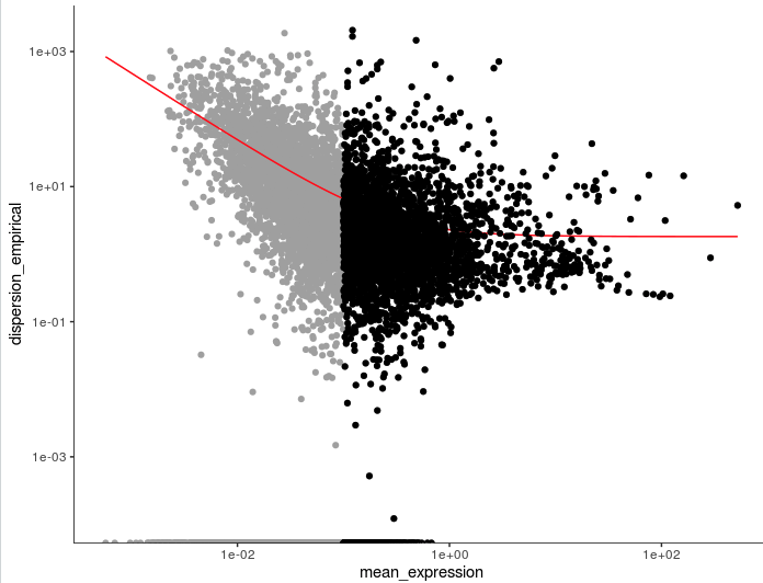
2. Monocle
参考:https://cole-trapnell-lab.github.io/monocle-release/docs/#clustering-cells
# V2
cds <- estimateSizeFactors(cds)
cds <- estimateDispersions(cds)
disp_table <- dispersionTable(cds)
> head(disp_table)
     gene_id mean_expression dispersion_fit dispersion_empirical
1 AL669831.5     0.011673004      42.669671             0.000000
2      NOC2L     0.140316168       5.221419             1.696712
3    PLEKHN1     0.016292004      31.089206             0.000000
4 AL645608.8     0.009537725      51.814220             0.000000
5       HES4     0.265523990       3.619078            28.119205
6      ISG15     0.793811626       2.424032            11.047583

unsup_clustering_genes <- subset(disp_table, mean_expression >= 0.1)
cds <- setOrderingFilter(cds, unsup_clustering_genes$gene_id)
plot_ordering_genes(cds)
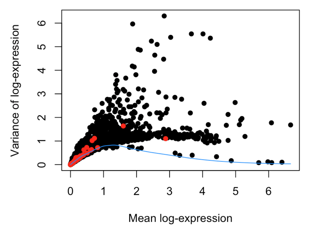
3. scran
参考:https://bioconductor.riken.jp/packages/3.7/workflows/vignettes/simpleSingleCell/inst/doc/work-5-mnn.html
利用函数trendVar()和decomposeVar() 根据表达量计算highly variable genes (HVGs)
fit <- trendVar(sce, parametric=TRUE)
dec <- decomposeVar(sce, fit)
如果有不感兴趣的差异来源(例如plate、donor),为了确保后面鉴定HVGs过程不会扩大真实的数据偏差,可以设置block
block <- paste0(sce$Plate, "_", sce$Donor)
fit <- trendVar(sce,block=block, parametric=TRUE)
dec <- decomposeVar(sce, fit)
最后作图
plot(dec$mean, dec$total, xlab="Mean log-expression",
    ylab="Variance of log-expression", pch=16)
OBis.spike <- isSpike(sce)
points(dec$mean[is.spike], dec$total[is.spike], col="red", pch=16)
curve(fit$trend(x), col="dodgerblue", add=TRUE)
在
decomposeVar函数帮助文档中有一句描述:Highly variable genes (HVGs) can be identified as those with large biological components. The biological component is determined by subtracting the technical component from the total variance.“HVGs能够代表大部分的生物学差异,而这种差异是由总体差异减去技术因素差异得到的”
dec$Symbol <- rowData(dec)$Symbol
dec <- dec[order(dec$bio, decreasing=TRUE),]

> head(dec,2)
DataFrame with 2 rows and 7 columns
                            mean            total              bio
                       <numeric>        <numeric>        <numeric>
ENSG00000254647 2.83712754306791 6.30184692631371 5.85904290864641
ENSG00000129965 1.88188510741958 5.96360144483475  5.5152391307155
                             tech   p.value       FDR      Symbol
                        <numeric> <numeric> <numeric> <character>
ENSG00000254647 0.442804017667299         0         0         INS
ENSG00000129965 0.448362314119254         0         0    INS-IGF2
4. M3Drop
Brennecke et al. (2013) Accounting for technical noise in single-cell RNA-seq experiments. Nature Methods 10, 1093-1095. doi:10.1038/nmeth.2645
library(M3DExampleData)
# 需要提供表达矩阵(expr_mat)=》normalized or raw (not log-transformed)
HVG <- M3Drop::BrenneckeGetVariableGenes(expr_mat=M3DExampleData, spikes=NA, suppress.plot=FALSE, fdr=0.1, minBiolDisp=0.5, fitMeanQuantile=0.8)
HVG_spike <- BrenneckeGetVariableGenes(Mmus_example_list$data, spikes=5550:5600)
5. 自定义函数
Extract genes with a squared coefficient of variation >2 times the fit regression (Brennecke et al 2013 method) 实现了:Select the highly variable genes based on the squared coefficient of variation and the mean gene expression and return the RPKM matrix the the HVG
getMostVarGenes <- function(
  data=data,				# RPKM matrix
  fitThr=1.5, 			# Threshold above the fit to select the HGV
  minMeanForFit=1			# Minimum mean gene expression level
){
  # data=females;fitThr=2;minMeanForFit=1
  # Remove genes expressed in no cells
  data_no0 <- as.matrix(
    data[rowSums(data)>0,]
  )
  # Compute the mean expression of each genes
  meanGeneExp <- rowMeans(data_no0)
  names(meanGeneExp)<- rownames(data_no0)

  # Compute the squared coefficient of variation
  varGenes <- rowVars(data_no0)
  cv2 <- varGenes / meanGeneExp^2

  # Select the genes which the mean expression is above the expression threshold minMeanForFit
  useForFit <- meanGeneExp >= minMeanForFit

  # Compute the model of the CV2 as a function of the mean expression using GLMGAM
  fit <- glmgam.fit( cbind( a0 = 1,
                            a1tilde = 1/meanGeneExp[useForFit] ),
                     cv2[useForFit] )
  a0 <- unname( fit$coefficients["a0"] )
  a1 <- unname( fit$coefficients["a1tilde"])

  # Get the highly variable gene counts and names
  fit_genes <- names(meanGeneExp[useForFit])
  cv2_fit_genes <- cv2[useForFit]
  fitModel <- fit$fitted.values
  names(fitModel) <- fit_genes
  HVGenes <- fitModel[cv2_fit_genes>fitModel*fitThr]
  print(length(HVGenes))

  # Plot the result
  plot_meanGeneExp <- log10(meanGeneExp)
  plot_cv2 <- log10(cv2)
  plotData <-  data.frame(
    x=plot_meanGeneExp[useForFit],
    y=plot_cv2[useForFit],
    fit=log10(fit$fitted.values),
    HVGenes=log10((fit$fitted.values*fitThr))
  )
  p <- ggplot(plotData, aes(x,y)) +
    geom_point(size=0.1) +
    geom_line(aes(y=fit), color="red") +
    geom_line(aes(y=HVGenes), color="blue") +
    theme_bw() +
    labs(x = "Mean expression (log10)", y="CV2 (log10)")+
    ggtitle(paste(length(HVGenes), " selected genes", sep="")) +
    theme(
      axis.text=element_text(size=16),
      axis.title=element_text(size=16),
      legend.text = element_text(size =16),
      legend.title = element_text(size =16 ,face="bold"),
      legend.position= "none",
      plot.title = element_text(size=18, face="bold", hjust = 0.5),
      aspect.ratio=1
    )+
    scale_color_manual(
      values=c("#595959","#5a9ca9")
    )
  print(p)

  # Return the RPKM matrix containing only the HVG
  HVG <- data_no0[rownames(data_no0) %in% names(HVGenes),]
  return(HVG)
}
P.S.
参考:https://bioconductor.org/packages/release/workflows/vignettes/simpleSingleCell/inst/doc/var.html https://bioconductor.org/packages/devel/bioc/vignettes/scran/inst/doc/scran.html
还有其他的一些函数:
- the coefficient of variation, using the
technicalCV2()function (Brennecke et al. 2013) or theDM()function (Kim et al. 2015) in scran, which quantify expression variance based on the coefficient of variation of the (normalized) counts. 另外还有technicalCV2()的升级版improvedCV2() - the dispersion parameter in the negative binomial distribution, using the
estimateDisp()function in edgeR (McCarthy, Chen, and Smyth 2012). - a proportion of total variability, using methods in the BASiCS package (Vallejos, Marioni, and Richardson 2015).