162-一个看似简单的需求——修改富集分析的dotplot图
刘小泽写于2020.2.6 最近再一次做起了转录组,但这一次需求有点小改变,需要自己定制一下,具体原因看本文吧。其中要特别表扬花花💏同学,帮了个大忙!
问题由来
我们一般进行富集分析,一般的做法都是:
# 先得到上调的差异基因gs_up,可以先不进行pvalue、qvalue的过滤
up <- enrichGO(gene          = gs_up,
               keyType       = 'ENSEMBL',
               OrgDb         = org.Hs.eg.db,
               ont           = "BP",
               pAdjustMethod = "BH",
               pvalueCutoff  = 1,
               qvalueCutoff  = 1,
               readable      = TRUE)
dotplot(up, showCategory=10,title="EnrichmentGO_BP")
得到的结果默认是:
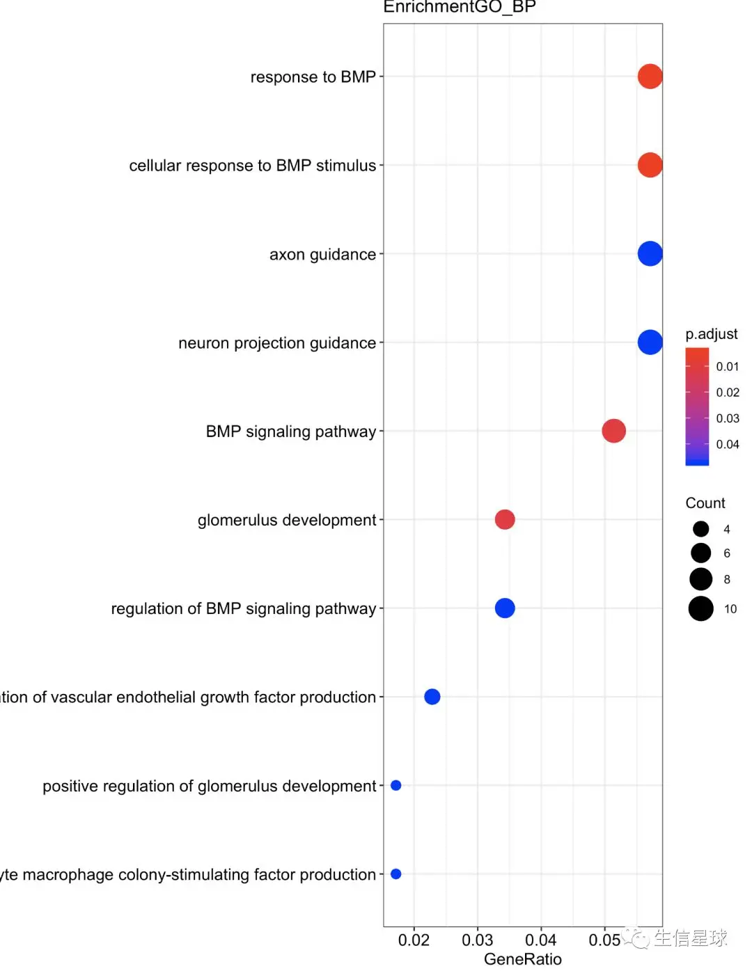
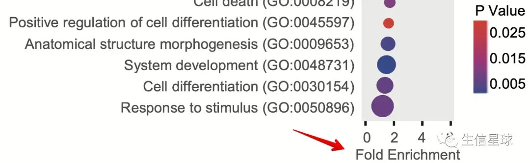
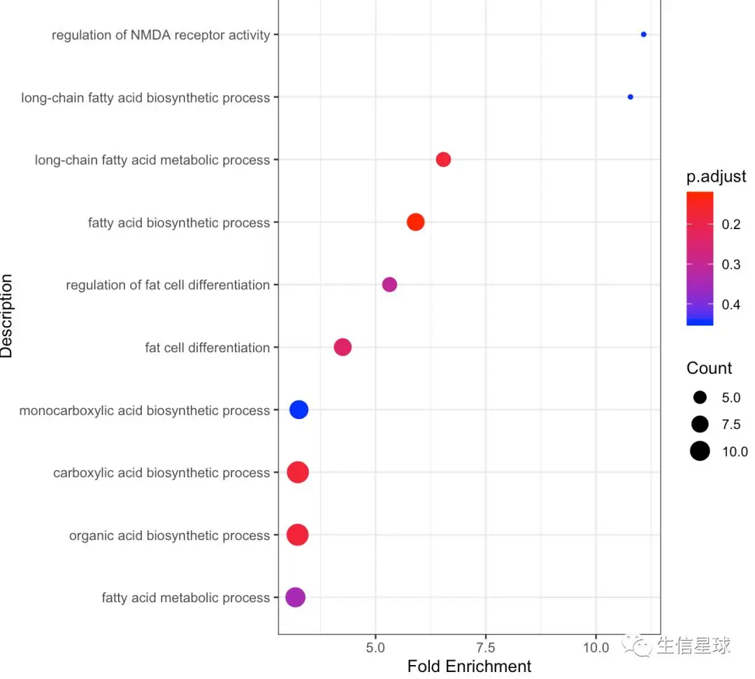
现在,想把横坐标进行改变,改成:Fold Enrichment,像这种图
什么是Fold Enrichment?和原来的GeneRatio啥关系?
看这里:https://yulab-smu.github.io/clusterProfiler-book/chapter13.html
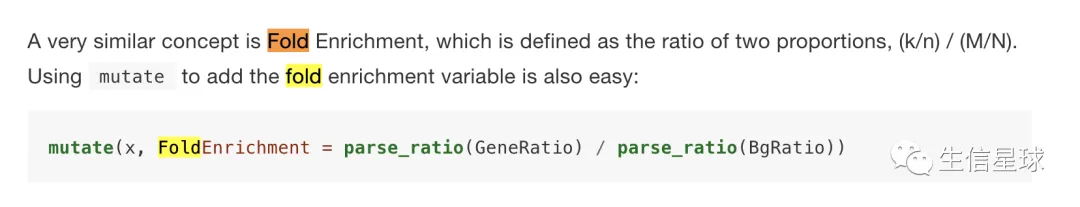
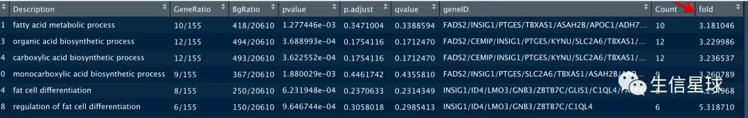
实际上,Fold Enrichment也是一个比值,是在原来GeneRatio的基础上,再除以BgRatio。
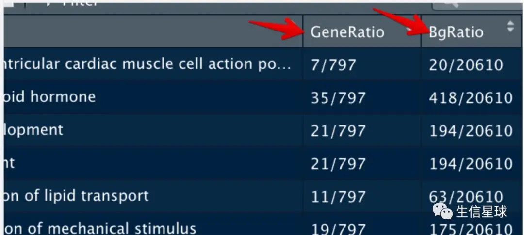
如下图,以第一行为例,默认情况下,dotplot给出的横坐标上,它会显示:7/797=0.0087
如果要改成Fold Enrichment,就是:(7/797)/(20/20610)=90.51
那么如何改变横坐标?
感觉很简单的样子,只要自己计算出来Fold Enrichment,然后加到原来数据中就好了。但是dotplot不太容易定制,它只支持GeneRatio or Count
看说明书:https://bioconductor.org/packages/devel/bioc/manuals/enrichplot/man/enrichplot.pdf

不过,好在Y叔的函数都是基于ggplot2的,于是我们可以自己拿到数据去作图
尝试第一步 准备作图数据
# 之前计算的结果
up <- enrichGO(gene          = gs_up,
               keyType       = 'ENSEMBL',
               OrgDb         = org.Hs.eg.db,
               ont           = "BP",
               pAdjustMethod = "BH",
               pvalueCutoff  = 1,
               qvalueCutoff  = 1,
               readable      = TRUE)
# 根据显著性取前10个
test=as.data.frame(up)
test=test[1:10,]
# 然后自己计算Fold Enrichment,并按照Fold Enrichment升序排序
library(stringr)
gr1 <- as.numeric(str_split(test$GeneRatio,"/",simplify = T)[,1])
gr2 <- as.numeric(str_split(test$GeneRatio,"/",simplify = T)[,2])
bg1 <- as.numeric(str_split(test$BgRatio,"/",simplify = T)[,1])
bg2 <- as.numeric(str_split(test$BgRatio,"/",simplify = T)[,2])
test$fold <- (gr1/gr2)/(bg1/bg2)
test <- arrange(test,fold)
尝试第二步 作图
使用最简单的作图代码
ggplot(test,aes(x = fold,y = Description))+
    geom_point(aes(color = p.adjust,
                   size = Count))+
    scale_color_gradient(low = "red", high = "blue")+
    xlab("Fold Enrichment")+
    theme_bw()
结果出来是这样:

尝试修改
虽然结果出来了,但总感觉怪怪的,没有按照一个顺序排列。
这里花花给出了最大的帮助,她一眼(可能是两眼)就看到了,虽然X轴是从小到大排列,但Y轴不是,它是按照首字母的顺序进行的排列,所以结果是乱的
于是她帮我加了一行代码,将Y轴的Description设成有序型因子变量,
test$Description = factor(test$Description,levels = test$Description,ordered = T)
实际上将我已经按照Fold Enrichment排序好的数据框保持原样,并且其中的Description同样按照从上到下的顺序进行了排列
比如原来的Description是字符型变量,作图默认按照字母顺序,也就是carboxylic这一条会是第一个,但现在按照Fold Enrichment排序后,它到了第3位。我们就顺势把这个carboxylic设成有序型因子,它现在就不再是一个字符串了,而是按照一个数3进行后面的排列【这里看不懂也没啥关系,反之因子型的概念就是有点绕】:

这个修改完之后,再次运行作图代码:

完事了吗?好像还差一点!
好像图例中这个p.adjust的顺序有点…强迫症犯了,最好是从小到大排列
于是,搜索了一下,找到了答案(https://stackoverflow.com/questions/22458970/how-to-reverse-legend-labels-and-color-so-high-value-starts-downstairs):
ggplot(test,aes(x = fold,y = Description))+
    geom_point(aes(color = p.adjust,
                   size = Count))+
    scale_color_gradient(low = "red", high = "blue")+
    xlab("Fold Enrichment")+
    theme_bw()+
    #edit legends
    guides(
        #reverse color order (higher value on top)
        color = guide_colorbar(reverse = TRUE))
        #reverse size order (higher diameter on top)
        #size = guide_legend(reverse = TRUE))
嗯,这回感觉清爽多了