169-跟着刘小泽一起探索可变剪切分析
刘小泽写于2020.2.23
上午接到一个求助,让我帮忙分析可变剪切。无奈这个名词听得多,用得少。但不能怂,学起来。于是今天用了半天时间搜集整理各种资料,6种方法汇集成一篇,思路也逐渐清晰起来…
介绍
概念介绍
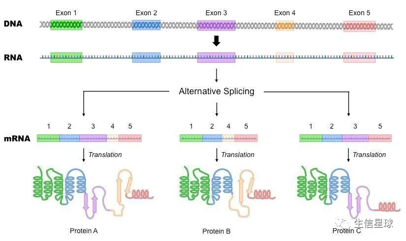
可变剪接(Alternative splicing)是基因表达的一种调节方式。真核细胞的基因序列中,包含了内含子与外显子,两者交互穿插。一般来说,内含子在基因转录成mRNA前体后会被RNA剪接体移除,剩下的外显子才是能够存在于成熟mRNA(之后再进一步转译成蛋白质)的片段。一条未经剪接的RNA,含有的多种外显子被剪成的不同组合,可转译出不同的蛋白质。这样保证了:同一基因中的外显子以不同形式进行组合,使一个基因在不同时间、不同环境中能够制造出不同的蛋白质,增加生理状况下系统的复杂性或适应性。
其他解释:
1:有些基因的一个mRNA前体通过不同的剪接方式(选择不同的剪接位点)产生不同的mRNA剪接异构体(isoform),这一过程称为可变剪接(或选择性剪接,alternative splicing)
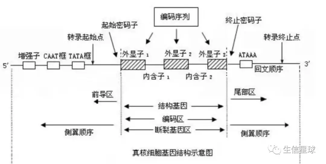
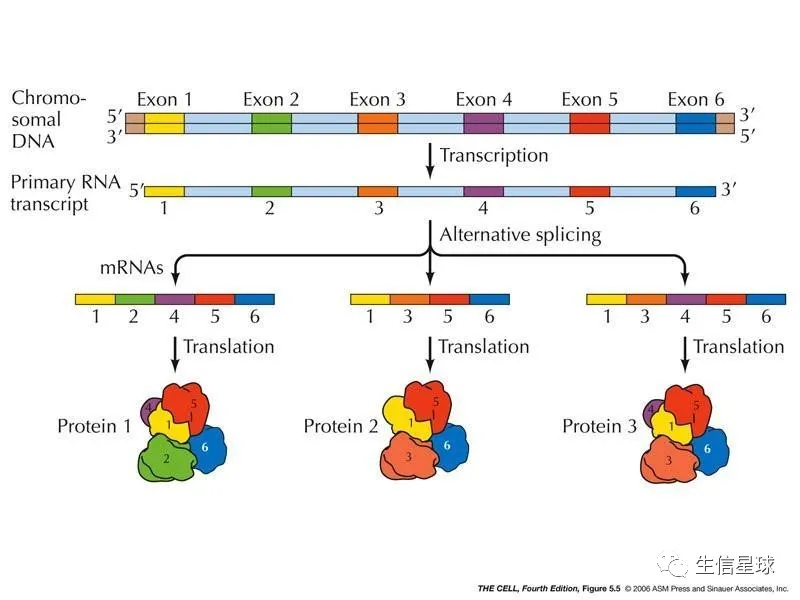
2:转录组一般是指从细胞或组织的基因组所转录出来的RNA的总和,包括编码蛋白质的mRNA和各种非编码RNA(rRNA,tRNA,snRNA,snoRNA,lncRNA,microRNA等)。真核生物的基因结构是不连续的。基因组最初的转录产物其实并不是成熟的mRNA分子,而是它的前体pre-mRNA,那么怎么变成成熟的mRNA呢?
就需要从pre-mRNA中将非编码蛋白质的内含子(intron)切除,然后拼接剩下的编码蛋白质的外显子(exon)。但实际上,在这个过程中,有多种多样的前切和拼接方式,从而产生不同的剪切异构体,即可变剪切事件。
**施一公在2017未来科学大奖颁奖典礼发表主题演讲:**剪接过程如此之复杂,你需要七个不同的剪接体,准确的识别内含子,把外显子拼在一起,这个过程很容易出错。 目前人类35%的遗传疾病或由RNA选择性剪接导致,比如视网膜色素变性、脊髓性肌肉萎缩症等。目前已有针对剪接体的药物被美国食品药品检验局批准上市,价格昂贵但非常有效 http://tech.sina.com.cn/2017-10-29/doc-ifynhhay8118096.shtml
人基因组中,大约95%的多外显子基因存在可变剪接。单独一个基因通过可变剪接产生十几种剪接异构体的现象很常见。最突出的例子是果蝇的Dscam基因,其潜在的可变剪接类型有38016个。
与疾病相关的几种典型剪接变异:
点突变–地中海贫血
与疾病相关的短重复元件突变–Alport综合症
单核苷酸多态性–阿兹海默症
可变剪接产生蛋白质亚型的比例改变–神经退化性疾病
剪接因子的缺失–脊髓型肌萎缩
研究进展:https://www.nature.com/subjects/alternative-splicing
一篇介绍AS机制的文献: Mechanism of alternative splicing and its regulation
类型介绍
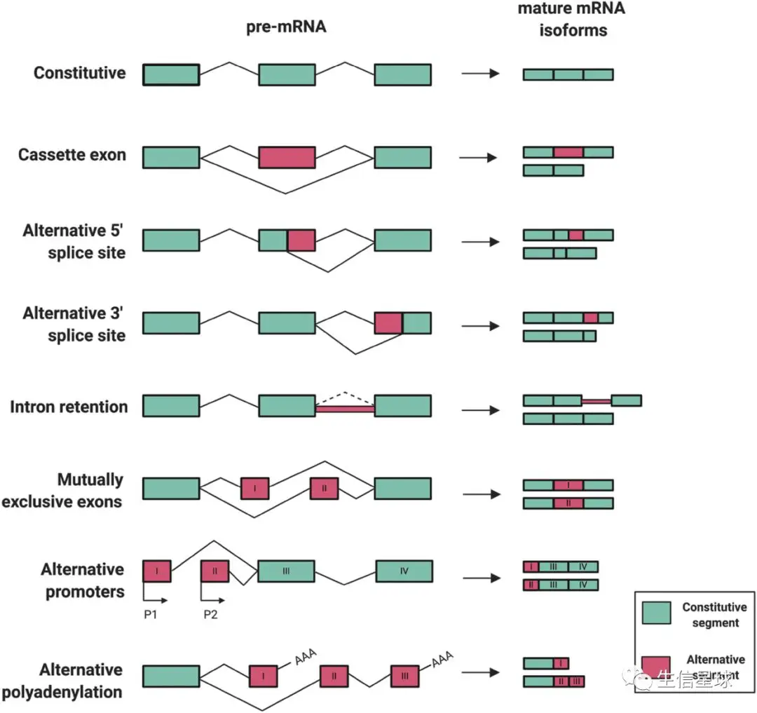
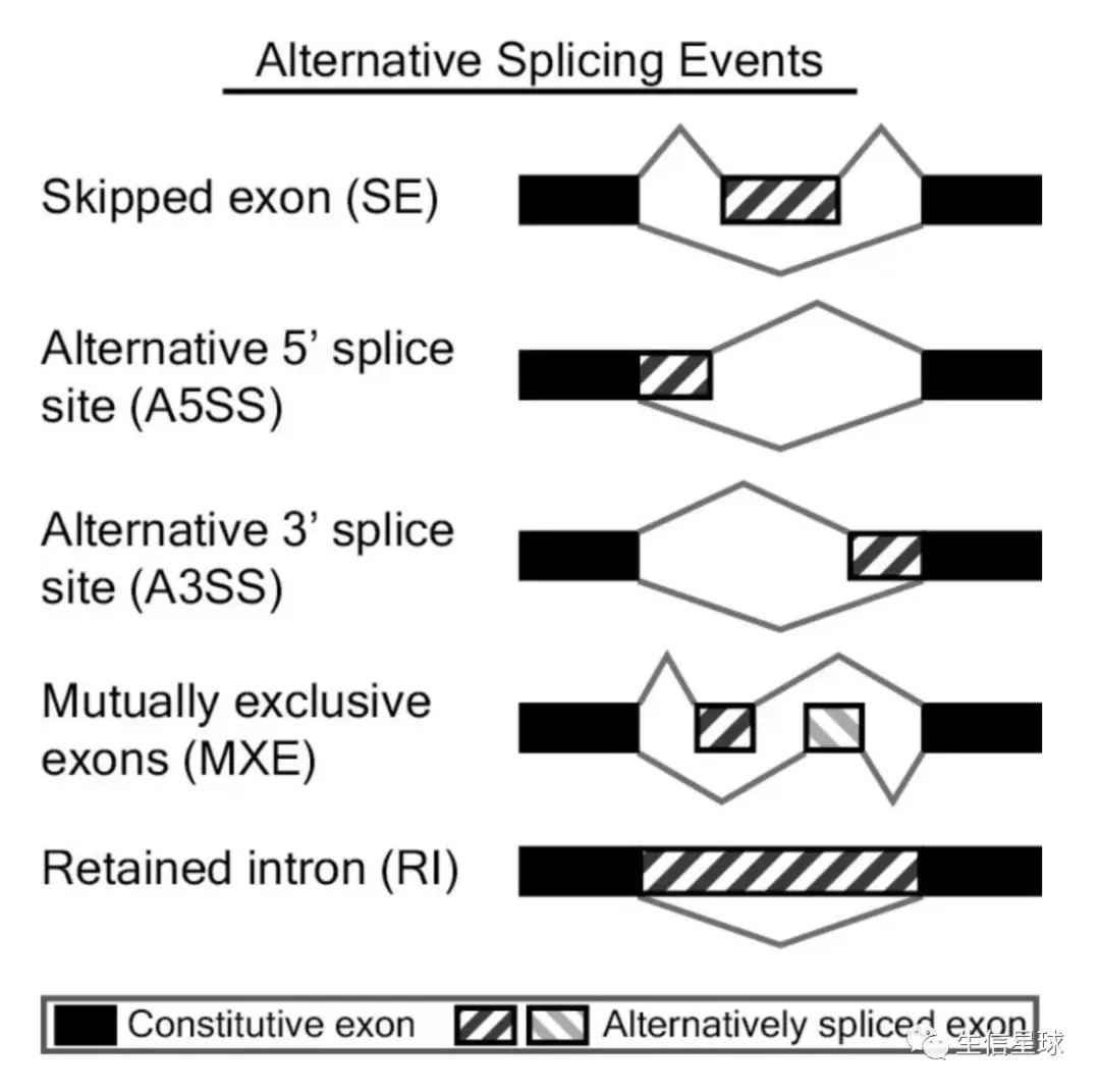
可变剪接是调节基因表达和产生蛋白质组多样性的重要机制,是导致真核生物基因和蛋白质数量较大差异的重要原因。在生物体内,主要存在7种可变剪接类型:
- ES(Exon skipping):外显子跳跃。外显子在前体mRNA剪接形成成熟mRNA过程中被跳过,最终没有出现在某些成熟mRNA上【发生跳跃的外显子和其两侧的内含子都被剪切掉;上游和下游的外显子被直接连着一起保留在剪切后的产物中】
- RI(Retained intron):内含子保留。前体mRNA在剪接形成成熟mRNA的过程中,部分内含子被保留下来【某一段核苷酸序列在一个剪切体中是外显子的一部分,而在与之对照的剪切体中却是内含子而被剪切掉】
- AD(Alternate Donor site)或A5SS(Alternative 5’ splice site):5’端可变剪接。前体mRNA在剪接形成成熟mRNA的过程中,5’端边界发生不同方式的剪接,导致5‘端外显子有所延长
- AA(Alternate acceptor site)或A3SS(Alternative 3’ splice site):3’端可变剪接。前体mRNA在剪接形成成熟mRNA的过程中,3’端边界发生不同方式的剪接,导致3‘端外显子有所延长
- AT(Alternate terminator)或Alternative last exon:第一个外显子发生改变
- AP(Alternate promoter)或Alternative first exon:最后一个外显子发生改变
- ME(Mutually exclusive exon):外显子选择性跳跃。形成的两种不同的转录本中,两转录本之间相同的外显子称为constitutive exon, 不同的外显子称为inclusive exon,inclusive exon不能同时存在与同一转录本中, 只能分别存在于不同转录本中
分析工具
1=> rMATS
介绍
网站:http://rnaseq-mats.sourceforge.net/
目前最新版是4.0.2
之前叫MATS(Multivariate Analysis of Transcript Splicing),后来为了有生物重复的RNA-Seq又升级到rMATS,相比之前的3.2.5版本,计算速度提升,并可支持多线程执行

它能识别5种AS事件:
安装
默认官网安装十分复杂:需要检测各种python,还需要sudo apt-get等等root权限。但十有八九最后还是会遇到一个问题: error while loading shared libraries: libgsl.so.0: cannot open shared object file: No such file or directory。此时依然是需要root安装一个库
使用:
sudo apt-get install libgsl0-dev解决方案依然是需要root:https://www.biostars.org/p/336864/
直接conda安装:
conda install -c bioconda rmats rmats2sashimiplot star
安装好检测:
rmats.py --help
用法说明如下:

使用示例
下载官网的示例数据:
mkdir ~/biosoft/rmats_v4.0.2 && cd ~/biosoft/rmats_v4.0.2
# -O 指定以不同文件名保存
wget https://sourceforge.net/projects/rnaseq-mats/files/MATS/testData.tgz/download -O testData.tgz
# 然后解压
tar xvzf testData.tgz

4.5M Aug 15  2016 231ESRP.25K.rep-1.R1.fastq
4.5M Aug 15  2016 231ESRP.25K.rep-1.R2.fastq
2.6M Apr 26  2018 231ESRP.25K.rep-1.bam
4.6M Aug 15  2016 231ESRP.25K.rep-2.R1.fastq
4.6M Aug 15  2016 231ESRP.25K.rep-2.R2.fastq
2.6M Apr 26  2018 231ESRP.25K.rep-2.bam
4.5M Aug 15  2016 231EV.25K.rep-1.R1.fastq
4.5M Aug 15  2016 231EV.25K.rep-1.R2.fastq
2.6M Apr 26  2018 231EV.25K.rep-1.bam
4.6M Aug 15  2016 231EV.25K.rep-2.R1.fastq
4.6M Aug 15  2016 231EV.25K.rep-2.R2.fastq
2.6M Apr 26  2018 231EV.25K.rep-2.bam
  44 Apr 26  2018 b1.txt
  40 Apr 26  2018 b2.txt
 108 Apr 26  2018 s1.txt
 100 Apr 26  2018 s2.txt
软件支持两种格式输入,文件内以逗号分隔重复样本名:
使用fastq测序数据:这样的话需要用
--s1、--s2分别指定两个样本的fq文件名,这样方便了自己,不需要自己运行STAR比对,直接用fq文件出结果。但需要自己下载安装STAR和比对的索引文件Obtain STAR genome index for genome by either of the following two ways:
Download pre-built STAR indexes if using Human (hg38, hg19) or Mouse (mm10). 【hg38、hg19、mm10有现成的可以下载:http://labshare.cshl.edu/shares/gingeraslab/www-data/dobin/STAR/STARgenomes/】
Build your own STAR index following STAR manual from genome fasta sequence【自己构建的话:https://github.com/alexdobin/STAR/tree/master/doc】
使用比对后的bam:它支持其他比对软件(如tophat、hisat2等)作为输入,从而减少rMATS的运行时间
如果直接使用fastq测序数据
# 测试数据中已经帮我们准备好了名称
cat s1.txt
231ESRP.25K.rep-1.R1.fastq:231ESRP.25K.rep-1.R2.fastq,231ESRP.25K.rep-2.R1.fastq:231ESRP.25K.rep-2.R2.fastq

cat s2.txt
231EV.25K.rep-1.R1.fastq:231EV.25K.rep-1.R2.fastq,231EV.25K.rep-2.R1.fastq:231EV.25K.rep-2.R2.fastq
我们自己需要准备好GTF文件和STAR index,然后:
# 打开下面👇链接
# GTF和STAR for hg19:
http://labshare.cshl.edu/shares/gingeraslab/www-data/dobin/STAR/STARgenomes/ENSEMBL/homo_sapiens/ENSEMBL.homo_sapiens.release-75/

# GTF和STAR for hg38:
http://labshare.cshl.edu/shares/gingeraslab/www-data/dobin/STAR/STARgenomes/ENSEMBL/homo_sapiens/ENSEMBL.homo_sapiens.release-83/

# 如果运行STAR
STAR --readFilesIn test_1.clean.fq test_2.clean.fq \
--chimSegmentMin 2 \
--outFilterMismatchNmax 3 \
--alignEndsType EndToEnd \
--runThreadN 5 \
--outSAMstrandField intronMotif \
--outSAMtype BAM SortedByCoordinate \
--alignSJDBoverhangMin 6 \
--alignIntronMax 299999 \
--genomeDir /YOUR_INDEX_DIR/ \
--sjdbGTFfile /YOUR_GTF_DIR/ \
--outFileNamePrefix test

# 然后运行rmats
rmats.py --s1 s1.txt --s2 s2.txt --gtf gtf/Homo_sapiens.Ensembl.GRCh37.72.gtf --bi ~/STARindex/hg19 --od out_test -t paired --nthread 6 --readLength 50 --tophatAnchor 8 --cstat 0.0001 --tstat 6
如果直接使用bam测序数据
# 测试数据中已经帮我们准备好了名称
cat b1.txt
231ESRP.25K.rep-1.bam,231ESRP.25K.rep-2.bam

cat b2.txt
231EV.25K.rep-1.bam,231EV.25K.rep-2.bam
只需要提供GTF即可:
rmats.py --b1 b1.txt --b2 b2.txt --gtf ~/reference/gtf/ensembl/hg19/Homo_sapiens.GRCh37.75.gtf --od bam_test -t paired --readLength 50 --cstat 0.0001 --libType fr-unstranded
看一些参数的意思
-t readType 双端测序为paired,单端测序为single
--readLength 测序reads的长度(这里测试数据的长度是51)
--gtf 指定GTF文件
--od 指定输出目录
--nthread 设置线程数
--cstat 设置一小数 (the cutoff splicing difference,default is 0.0001 for 0.01% difference. Valid: 0 ≤ cutoff < 1)【它采用的是Likelihood-ratio test来比较两组样本可变剪切是否有差异】
-libType 默认是非链特异性(fr-unstranded);如果使用特异性文库,可以指定fr-firststrand或者fr-secondstrand
结果文件
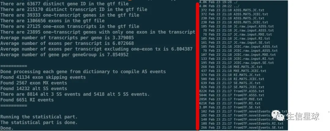
结果的解读看:https://cloud.tencent.com/developer/article/1366294
可视化
使用rmats2sashimiplot
需要注意:
- 如果直接使用rMATS从fastq输入文件到结果输出文件,那么rMATS是不保留中间的bam文件的
- rmats2sashimiplot可视化则需要bam文件作为输入,因此最好自己先进行一轮比对,然后进行rMATS,最后再plot
- 使用的bam文件要先用samtools对bam文件建索引,否则
rmats2sashimiplot会自己再做一遍,而且很慢 - 确保rMATS的结果文件中染色体和bam文件的染色体名称一致(要么都是chr1,要么都是直接数字1)
- 出图结果默认是PDF
# 以单端为例
rmats2sashimiplot --b1 A1.bam,A2.bam,A3.bam \
--b2 B1.bam,B2.bam,B3.bam \
-t SE \
-e ./SE.MATS.JC_top20.txt \
--l1 A --l2 B \
--exon_s 1 --intron_s 1 \
-o SE_plot
2 => CircSplice
介绍
http://gb.whu.edu.cn/CircSplice/
circRNA作为一个新兴的非编码RNA,也同样通过mRNA前体的可变剪切而来。作者建议:测序数据文库最好采用去rRNA及线性RNA。
目前常用的可变剪切事件预测软件有 CIRI-full (更适合长片段,>250或300bp),以及短片段的CIRI-AS (50~150bp),但是并没有提供样本间比较的功能。
它是一款基于perl编写的流程,能够通过预测反向剪切事件识别circRNA,支持 GT-AG和CT-AC两种剪切位点。提供四种circ-AS事件类型结果:外显子跳跃(SE),内含子保留(RI),5’端可变剪接(A5SS)和3’端可变剪接(A3SS)
1 质控及过滤
fastqc Sample.R1.fq.gz Sample.R2.fq.gz
trim_galore -q 20 --phred33 --stringency 3 --length 20 -e 0.1 --paired Sample.R1.fq Sample.R2.fq --gzip -o Sample
fastqc Sample.R1_trimmed.fq.gz Sample.R2_trimmed.fq.gz
2 比对
# 建索引
STAR --runThreadN NumberOfThreads --runMode genomeGenerate --genomeDir /path/to/genomeDir --genomeFastaFiles /path/to/genome/fasta1 /path/to/genome/fasta2 --sjdbGTFfile /path/to/annotations.gtf
# 比对
STAR --genomeDir /path/to/genomeDir --readFilesIn Sample.R1_trimmed.fq.gz Sample.R2_trimmed.fq.gz --readFilesCommand zcat --runThreadN 10 --chimSegmentMin 20 --chimScoreMin 1 --alignIntronMax 100000 --outFilterMismatchNmax 4 --alignTranscriptsPerReadNmax 100000 --outFilterMultimapNmax 2 --outFileNamePrefix Sample
3 鉴定
# For paired-end library,
CircSplice.pl Chimeric.out.sam hg38.genome.fa bed_refFlat_hg38.txt

# single-end library,
CircSplice-single.pl Chimeric.out.sam hg38.genome.fa bed_refFlat_hg38.txt
将获得两个结果文件,Chimeric.out.sam.result.as(circ-As时间)和Chimeric.out.sam.result.circ(circRNA鉴定)
4 合并结果
CircSplice-merge.pl dir-as dir-circ
CircSplice-merge merges results according to the genomic coordinates with 2bp mismatch toleration.
得到结果
详细的结果见:http://gb.whu.edu.cn/CircSplice/userguide.html
- AS_result 中每一行代表样本中的一个AS事件
- Circ_result 中每一行代表一条circRNA
其他物种
CircSplice.pl 也支持其他物种或者基因组的版本,需要自行构建,文本格式如下
Chromosome
Start coordinates -2
End coordinates +2
Transcript ID
Number of exons
Strand
Gene symbol
Transcript ID
Chromsome
Strand
Start coordinates
end coordinates
Start coordinates of CDS
End coordinates of CDS
Number of exons
Start coordinates of each exon
End coordinates of each exon
Gene type (lncRNA or mRNA)
再通过 reftobed.pl refFlat.txt转换bed-refFlat格式
3 => CASH
介绍
http://www.novelbio.com/cash/index.html
这是一款国产软件,全称:Comprehensive alternative splicing hunting
It aims to self-construct AS (alternative splicing) sites and detect differential AS events between samples of RNA-Seq data. 引用: Zhou X, Wu W, Li H, Cheng Y, Wei N, Zong J, Feng X, Xie Z, Chen D, and Manley JL et al. 2014. Transcriptome analysis of alternative splicing events regulated by SRSF10 reveals position-dependent splicing modulation. Nucleic Acids Res 42: 4019-4030.
包含了主要的两步: SpliceCons (Splice site Construction) and SpliceDiff (differential AS detection)
- SpliceCons increases the recognition of AS events considerably and subsequently
- SpliceDiff uses two combined statistical methods to improve the detection of differential AS events
需要提供的文件:比对产生的bam文件(必须经过sort + index)、GTF基因注释文件(另外,如果想找到剪切位点附近的序列,还需要上传基因组序列信息)
使用说明在:http://www.novelbio.com/cash/manual_index.html
下载地址在:http://www.novelbio.com/cash/cash/cash_v2.2.0.zip
参考数据在:http://www.novelbio.com/cash/cash/Examples.zip
下载好检查软件
unzip cash_v2.2.0.zip
cd cash_v2.2.0
# 需要提前用conda install -c anaconda openjdk -y
java -jar cash.jar --help
使用示例
java -jar -Xmx10g cash.jar \
--Case:Mutation file1.bam,file2.bam \
--Control:WildType file3.bam,file4.bam \
--GTF genes.gtf --Output outFilePrefix
需要JAVA环境:requires jre1.8 or later, and at least 8GB memory for 2vs2 human samples
关于结果

4 => 【R包】LeafCutter v0.2.8
文章在: Annotation-free quantification of RNA splicing using LeafCutter 特点:可省略GTF/GFF文件;可以检测splicing quantitative trait loci (sQTLs) 官网在:http://davidaknowles.github.io/leafcutter/ 参考:http://www.bio-info-trainee.com/2949.html
安装可以用
conda install -c davidaknowles r-leafcutter
# 或者直接在Rstudio
devtools::install_github("davidaknowles/leafcutter/leafcutter")
官方提供的一些脚本和测试数据在
git clone https://github.com/davidaknowles/leafcutter
cd leafcutter
## 其中有一个bam2junc.sh 一会要用到
首先:bam2junc
# $bam是bam名称; $sample.junc是生成的结果
bam2junc.sh  $bam $sample.junc
# 多个bam可以批量操作
# 会得到
chr11    109735445   109827551   .   19  +
chr18    48458730    48465939    .   8   -
chr12    82751048    82752457    .   12  -
chr15    51018323    51018517    .   14  -
然后:intron clustering
需要python 2.7
ls *.junc >test_juncfiles.txt

python leafcutter_cluster.py -j test_juncfiles.txt -m 50 -o test -l 500000
# 结果的**_perind_numers.counts.gz文件中,每一行是一个内含子,每一列是一个样本的表达值(然后利用这些数值进行可变剪切),例如:
chr8:145651155:145651305:clu_6538 21 14 19 8 9 0 13 33 0 0 4 0 5 8 12 0 12 34 15 0 0 10 11
接着:制作分组文件进行差异分析
分组文件就是两列:每个样本属于哪个组(有且只能有2个分组;如果分组很多可以多次处理多次运行),例如:
test1.bam control
test2.bam control
test3.bam trt
test4.bam trt
有了分组文件再运行
leafcutter_ds.R --num_threads 4 \
 --exon_file=~/leafcutter/data/gencode19_exons.txt.gz \
test_perind_numers.counts.gz group_info.txt
会得到:leafcutter_ds_cluster_significance.txt 【这个文件需要去理解】
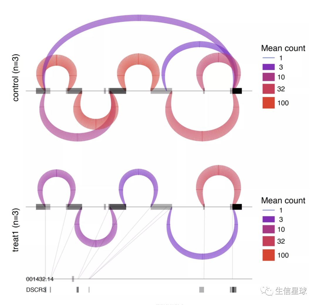
最后:可视化
ds_plots.R -e ~/leafcutter/data/gencode19_exons.txt.gz test_perind_numers.counts.gz group_info.txt leafcutter_ds_cluster_significance.txt -f 0.05
5 => 【R包】SGSeq
Splice event prediction and quantification from RNA-seq data 完全基于R语言处理 官方说明:https://bioconductor.org/packages/release/bioc/vignettes/SGSeq/inst/doc/SGSeq.html
参考:http://www.bio-info-trainee.com/2890.html
安装
if (!requireNamespace("BiocManager", quietly = TRUE))
    install.packages("BiocManager")

BiocManager::install("SGSeq")
需要的数据之bam
输入文件是bam(可以用hisat2、star等先比对好),然后构建好索引
当然,安装好这个包以后,也会有自带的测试数据
需要的数据之注释文件
通过 convertToTxFeatures()函数把 GRanges 对象转化成了一个TxFeatures对象
# for hg19 (这里使用chr16)
library(TxDb.Hsapiens.UCSC.hg19.knownGene)
txdb <- TxDb.Hsapiens.UCSC.hg19.knownGene
txdb <- keepSeqlevels(txdb, "chr16")
seqlevelsStyle(txdb) <- "NCBI"

# To work with the annotation in the SGSeq framework, transcript features are extracted from the TxDb object using function convertToTxFeatures()
txf_ucsc <- convertToTxFeatures(txdb)
txf_ucsc <- txf_ucsc[txf_ucsc %over% gr]
head(txf_ucsc)
type(txf_ucsc)
head(txName(txf_ucsc))
head(geneName(txf_ucsc))
这样就能标记下面五种类型了:
- J (splice junction)
- I (internal exon)
- F (first/5′-terminal exon)
- L (last/5′-terminal exon)
- U (unspliced transcript).
再用convertToSGFeatures() 把 TxFeatures 转成 SGFeatures
sgf_ucsc <- convertToSGFeatures(txf_ucsc)
head(sgf_ucsc)
SGFeatures对象包含了:
- J (splice junction)
- E (disjoint exon bin)
- D (splice donor site)
- A (splice acceptor site)
复杂一点的可视化 based on de novo prediction
sgfc_pred <- analyzeFeatures(si, which = gr)
head(rowRanges(sgfc_pred))
sgfc_pred <- annotate(sgfc_pred, txf_ucsc)
head(rowRanges(sgfc_pred))
df <- plotFeatures(sgfc_pred, geneID = 1, color_novel = "red")
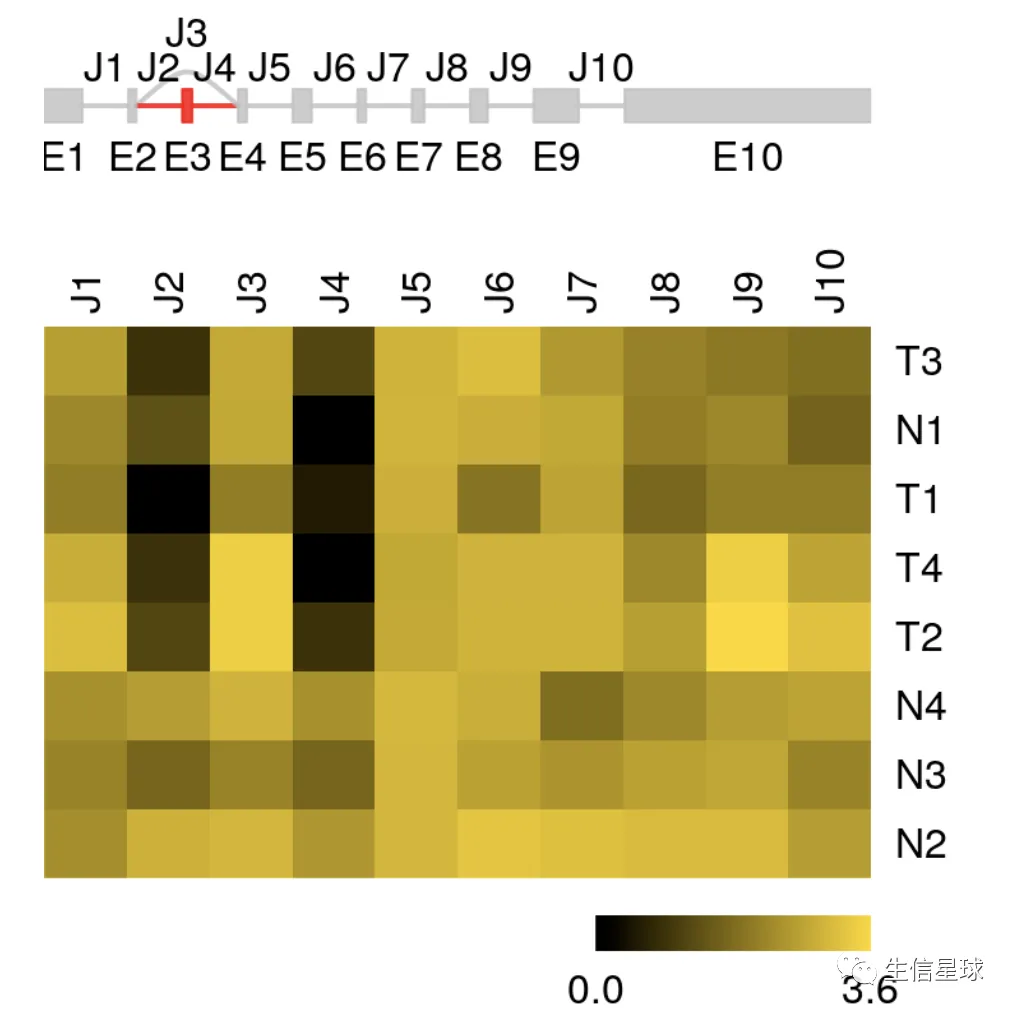
图中顶部灰色部分是:exons and splice junctions predicted from RNA-seq data are consistent with transcripts in the UCSC knownGene table
红色的是:an unannotated exon (E3, shown in red) was discovered from the RNA-seq data, which is expressed in three of the four normal colorectal samples (N2, N3, N4).
其他展现形式
# splice junctions
plotFeatures(sgfc_pred, geneID = 1, include = "junctions")
# exon bins
plotFeatures(sgfc_pred, geneID = 1, include = "exons")
# both exon bins and splice junctions
plotFeatures(sgfc_pred, geneID = 1, include = "both")
# 还能设置其他参数
# ”toscale“ controls which parts of the gene model are drawn to scale.
plotFeatures(sgfc_pred, geneID = 1, toscale = "gene")
plotFeatures(sgfc_pred, geneID = 1, toscale = "exon")
plotFeatures(sgfc_pred, geneID = 1, toscale = "none")
# 还有,【per-base read coverages】 and 【splice junction counts】 can be visualized with function plotCoverage()
par(mfrow = c(5, 1), mar = c(1, 3, 1, 1))
plotSpliceGraph(rowRanges(sgfc_pred), geneID = 1, toscale = "none", color_novel = "red")
for (j in 1:4) {
  plotCoverage(sgfc_pred[, j], geneID = 1, toscale = "none")
}

预测剪切异构体(splice variant)对蛋白编码的潜在影响
依然是先得到SGVariants这个对象再进行处理
# 鉴定Splice variant
sgvc_pred <- analyzeVariants(sgfc_pred)
sgvc_pred
mcols(sgvc_pred)

# 对Splice variant进行定量
variantFreq(sgvc_pred)
plotVariants(sgvc_pred, eventID = 1, color_novel = "red")

# 最后解释Splice variant
library(BSgenome.Hsapiens.UCSC.hg19)
seqlevelsStyle(Hsapiens) <- "NCBI"
vep <- predictVariantEffects(sgv_pred, txdb, Hsapiens)
vep
##   variantID     txName geneName                        RNA_change
## 1         2 uc002fjv.3    79791         r.88_89ins88+1798_88+1884
## 2         2 uc002fjw.3    79791     r.412_413ins412+1798_412+1884
## 3         2 uc010vot.2    79791 r.-105_-104ins-105+1798_-105+1884
##   RNA_variant_type                              protein_change
## 1        insertion   p.K29_L30insRINPRVKSGRFVKILPDYEHMAYRDVYTC
## 2        insertion p.K137_L138insRINPRVKSGRFVKILPDYEHMAYRDVYTC
## 3        insertion                                         p.=
##   protein_variant_type
## 1   in-frame_insertion
## 2   in-frame_insertion
## 3            no_change
结果的每行描述了:the effect of a particular splice variant on an annotated protein-coding transcript.
最后
SGSeq does not implement statistical tests for differential splice variant usage. However, existing software packages such as DEXSeq (Anders, Reyes, and Huber 2012) and limma (Ritchie et al. 2015) can be used for this purpose.
6 => 【R包】DEXSeq 通过外显子差异分析推测可变剪切
直接看:http://www.bio-info-trainee.com/bioconductor_China/software/DEXSeq.html 帮助文档在:http://bioconductor.org/packages/release/bioc/vignettes/DEXSeq/inst/doc/DEXSeq.html 官方建议:it is important to align them to the genome, not to the transcriptome, and to use a splice-aware aligner (i.e., a short-read alignment tool that can deal with reads that span across introns) such as TopHat2 (Kim et al. 2013), GSNAP (Wu and Nacu 2010), or STAR (Dobin et al. 2013)
首先安装包
## 首先安装包
# first prepare BioManager on CRAN
if(length(getOption("CRAN"))==0) options(CRAN="https://mirrors.tuna.tsinghua.edu.cn/CRAN/")
if(!require("BiocManager")) install.packages("BiocManager",update = F,ask = F)
if(length(getOption("BioC_mirror"))==0) options(BioC_mirror="https://mirrors.ustc.edu.cn/bioc/")

# use BiocManager to install
Biocductor_packages <- c('DEXSeq','pasilla')
for (pkg in Biocductor_packages){
    if (! require(pkg,character.only=T) ) {
        BiocManager::install(pkg,ask = F,update = F)
        require(pkg,character.only=T)
    }
}

suppressPackageStartupMessages(library("DEXSeq"))
suppressPackageStartupMessages(library("pasilla"))
准备3类输入文件=》1.counts矩阵
可以利用DEXSeq包中的python脚本得到
python /path/to/library/DEXSeq/python_scripts/dexseq_count.py Dmel.BDGP5.25.62.DEXSeq.chr.gff untreated1.sam untreated1fb.txt
有了这个外显子count文件,再看一下:
# 打开测试数据
inDir <- system.file("extdata", package="pasilla")
countFiles <- list.files(inDir, pattern="fb.txt$", full.names=TRUE)
countFiles
> ## 共七个样本,可以从文件名看到样本描述,即:每个基因的每个外显子的reads数量
> head(read.table(countFiles[1]))
               V1 V2
1 FBgn0000003:001  0
2 FBgn0000008:001  0
3 FBgn0000008:002  0
4 FBgn0000008:003  0
5 FBgn0000008:004  1
6 FBgn0000008:005  4
准备3类输入文件=》2.gtf格式的基因组注释文件
依然可以使用自带的python脚本制作:
python /path/to/library/DEXSeq/python_scripts/dexseq_prepare_annotation.py Drosophila_melanogaster.BDGP5.72.gtf Dmel.BDGP5.25.62.DEXSeq.chr.gff
看一下示例数据:
gffFile <- list.files(inDir, pattern="gff$", full.names=TRUE)
gffFile
准备3类输入文件=》3.实验设计表格
sampleTable <- data.frame(row.names=c(paste("treated", 1:3, sep=""), paste("untreated", 1:4, sep="")),
                          condition=rep(c("knockdown", "control"), c(3, 4)))
sampleTable
##            condition
## treated1   knockdown
## treated2   knockdown
## treated3   knockdown
## untreated1   control
## untreated2   control
## untreated3   control
## untreated4   control
构造DEXSeqDataSet对象
dxd <- DEXSeqDataSetFromHTSeq(
   countFiles,
   sampleData=sampleTable,
   design= ~sample + exon + condition:exon,
   flattenedfile=gffFile
   )

> dxd
class: DEXSeqDataSet
dim: 70463 14
metadata(1): version
assays(1): counts
rownames(70463): FBgn0000003:E001
  FBgn0000008:E001 ... FBgn0261575:E001
  FBgn0261575:E002
rowData names(5): featureID groupID exonBaseMean
  exonBaseVar transcripts
colnames: NULL
colData names(3): sample condition exon

> class(dxd)
[1] "DEXSeqDataSet"
attr(,"package")
[1] "DEXSeq"
差异分析
dxr <- DEXSeq(dxd) # 耗时
# 实际上做了以下几件事
if(F){
    dxd <- estimateSizeFactors(dxd)
    dxd <- estimateDispersions(dxd)
    dxd <- testForDEU(dxd)
    dxd <- estimateExonFoldChanges(dxd, fitExptoVar="condition")
    dxr1 <- DEXSeqResults(dxd)
}
指定基因进行可视化
## 最简单的图(红色部分是显著差异的外显子)
plotDEXSeq( dxr2, "FBgn0010909", legend=TRUE, cex.axis=1.2, cex=1.3, lwd=2 )
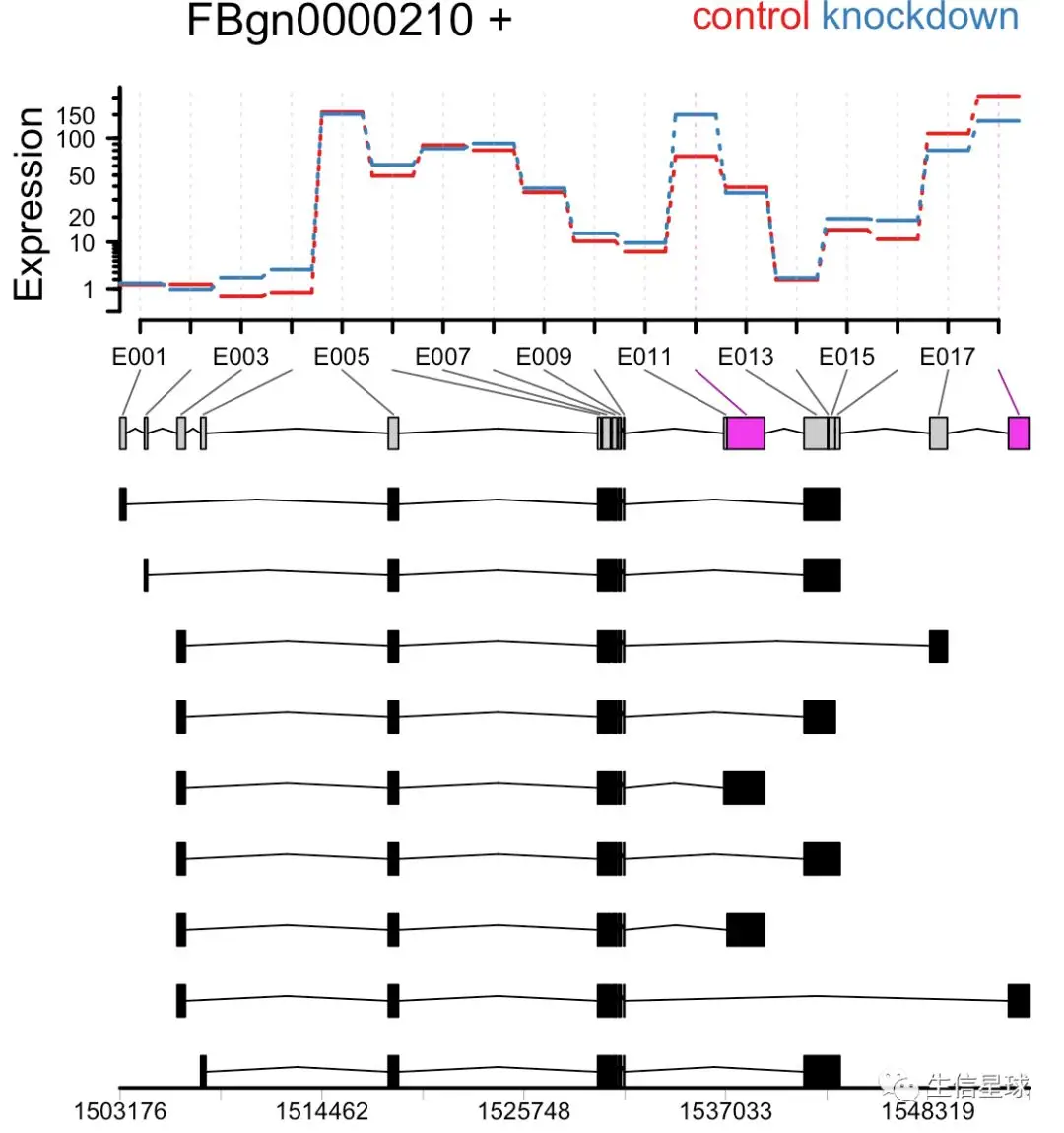
##将外显子表达量和转录本模型结合(putting differential exon usage results into the context of isoform regulation),这些转录本模型都是有注释的
plotDEXSeq( dxr, "FBgn0000210",
displayTranscripts=TRUE, legend=TRUE,
cex.axis=1.2, cex=1.3, lwd=2 )
# 按表达量查看(counts are normalized by dividing them by the size factors)
plotDEXSeq( dxr, "FBgn0000210",
expression=FALSE, norCounts=TRUE,
legend=TRUE, cex.axis=1.2,
cex=1.3, lwd=2 )
最后还能汇总,得到所有的显著性差异的基因图片
DEXSeqHTML( dxr, FDR=0.1, color=c("#FF000080", "#0000FF80") )
每一个都是能点开的
